Rural Revitalization and Integrated Urban-Rural Development

Spillover Effects of Green Development on Rural Revitalization: Based on Spatial Econometric Model and Complex Network

  • TANG Yuanxiu , 1, 2 ,
  • MA Jiali , 2, * ,
  • WANG Wenjie 2 ,
  • LI Shupeng 3
Expand
  • 1 School of Statistics and Mathematics, Zhejiang Gongshang University, Hangzhou 310018, China
  • 2 School of Big Data Statistics, Guizhou University of Finance and Economics, Guiyang 550025, China
  • 3 School of Computer Science, South China Normal University, Guangzhou 510631, China
* MA Jiali, E-mail:

TANG Yuanxiu, E-mail:

Received date: 2024-10-10

  Accepted date: 2025-05-10

  Online published: 2026-04-13

Supported by

The National Natural Science Foundation of China(12261016)

The Research Project of Higher Education Institutions in Guizhou Province for the Year 2023 (Youth Project)([2022]164)

The Research Project for Undergraduate Students at Guizhou University of Finance and Economics for the Year 2022(2022ZXSY034)

Abstract

In 2018, the Chinese government unveiled a comprehensive set of policies outlining the blueprint for rural revitalization, promoting the idea of “boosting rural revitalization through green development”. Using provincial panel data from 2011 to 2021, this study explores the impact of green development on rural revitalization, and the spatiotemporal and network evolution characteristics of this influence. Each region’s green development and rural revitalization levels are measured using the composite weighting method. Next, it explores the spatial characteristics of green development’s influence on rural revitalization by using spatial Durbin model. It further explores the heterogeneity of the spatial spillover effect of green development on rural revitalization using a two-regime spatial Durbin model. Lastly, it combines the complex network correlation method to identify important provinces.

Cite this article

TANG Yuanxiu , MA Jiali , WANG Wenjie , LI Shupeng . Spillover Effects of Green Development on Rural Revitalization: Based on Spatial Econometric Model and Complex Network[J]. Journal of Resources and Ecology, 2026 , 17(2) : 607 -619 . DOI: 10.5814/j.issn.1674-764x.2026.02.021

1 Introduction

Rural revitalization remains a crucial aspect of China’s development efforts. The Chinese government in 2022 notes that rural development remain a challenging aspect. Notably, it emphasizes leveraging green development for rural revitalization for synergistically advancing Chinese modernization. As a pivotal lever for resolving urban-rural development disparities, green development is reshaping rural revitalization pathways through the dual drivers of sustainable industrialization and industrial ecology (Li and Yu, 2024). However, considering China’s dual carbon goals and accelerated new urbanization, systematically understanding the spatial transmission mechanisms through which green development influences rural revitalization remains an urgent theoretical and practical imperative.
Despite a preliminary consensus on the linkage between green development and rural revitalization in China (Tang et al., 2024), two critical limitations persist in extant research: First, the predominant focus on county or urban agglomeration scales has overlooked the pivotal role of provincial-level units as network hubs (Wen et al., 2023). Second, methodological overreliance on conventional spatial econometric models reduces heterogeneous regional interactions to simplistic binary spatial adjacency. This not only inadequately quantifies gradient attenuation in green technology diffusion but also fails to identify polarization-trickle effects in cross-regional collaborative systems like the Beijing-Tianjin-Hebei and Yangtze River Delta regions (Suo and Leng, 2024).
Using panel data from 30 provincial-level regions in China from 2010 to 2022, this study innovatively integrates spatial econometrics and complex network analysis to systematically unravel the spatial spillover dynamics and network transmission pathways of green development on rural revitalization.
This study makes two contributions: Theoretically, it constructs a three-dimensional “local-neighbor-network” analytical framework, challenging the conventional linear assumption that spatial effects merely decay with geographic distance. Methodologically, our decomposition of the spillover matrix effects quantifies interprovincial green development spillovers, overcoming the rigid constraints of traditional adjacency matrices. Practically, it identifies “key nodal provinces” critical to green development, offering actionable insights for optimizing national green governance.
The subsequent sections proceed as follows: Section 2 systematically reviews the literature on green development and rural revitalization. Section 3 designs a multidimensional evaluation framework integrating the spatial econometric and network analysis models. Section 4 presents the empirical findings on three aspects: direct effects, spatial spillovers, and network topology. Section 5 outlines the theoretical contributions and practical implications, focusing on comparing our findings with the literature. Section 6 synthesizes our key conclusions, proposes institutional optimization directions aligned with the national unified market framework, and offers insights for advancing green development and rural revitalization strategies.

2 Literature review

2.1 Mechanisms and evolution of measurement methods

2.1.1 Dual pathways of theoretical mechanisms

In China, since Chinese policymakers proposed using green development to lead rural revitalization in the 2018 No. 1 Central Document, academic discussions on their relationship have evolved around two core pathways:
The first pathway is environmental governance. Based on a new structural economics perspective, Duan (2019) emphasized that environmental regulation tools, such as ecological restoration and pollution control, enhance rural governance efficiency, thereby promoting industrial organization and the value transformation of ecological products. Specifically, environmental governance reshapes rural production functions by reducing negative externalities and driving the transition from traditional to sustainable agriculture (Li and Yan, 2023). This pathway is empirically supported by Hu and Yue (2022), who found that a standard deviation increase in environmental regulation intensity boosts rural industrial value-added growth by 0.28%.
The second pathway is industrial transformation. Wang et al. (2021) proposed a “green technology-industrial upgrading-rural revitalization” transmission chain, arguing that green technological innovations reconstruct rural economic structures through the factor reallocation effect. Zhong et al. (2022) further revealed that eco-industrialization creates new employment opportunities. Notably, Xie and Feng (2023) identified spatial heterogeneity in this pathway: Compared with western regions, eastern regions with higher factor market maturity exhibited a stronger promotional effect of green technology diffusion on rural revitalization.
However, two limitations remain: First, most studies adopt linear regression models, neglecting the nonlinear threshold effects of green development. For instance, Fu and Xue (2024) noted that when rural human capital falls below a critical threshold, green technology investments exacerbate rural decline due to skill mismatches. Second, spatial interactions are understudied, with extant research considering regions as independent units while ignoring the network effects from factor mobility (Zhou et al., 2024).

2.1.2 Paradigm shifts in measurement systems

In measuring green development, single-dimensional indicators dominated early studies. Tao and Huang (2005) used energy consumption per unit of GDP to measure green efficiency but failed to capture emerging models like resource recycling. Multi-dimensional index systems emerged next. Li and Pan (2011) developed a system with four first-tier indicators. However, the equal-weight assignments distorted weights for heterogeneous indicators like forest coverage and industrial solid waste utilization rates. Dynamic composite weighting methods are now gaining traction. Tang et al.’s (2024) time-decay entropy-analytic hierarchy process (AHP) method aligns weight allocations with the cumulative effects of green development in panel data (2011- 2020).
For rural revitalization assessment, Mao’s (2021) “Five Dimensions” index system aligns with policy frameworks but suffers from some issues: 1) An overreliance on traditional agricultural metrics under the “industrial prosperity” dimension neglects new formats like tertiary integration; 2) Critical indicators, such as ecological product value conversion rates, are missing in the “ecological livability” dimension.

2.2 Paradigm shifts in spatial effects research

Traditional spatial econometric models analyze spillovers using geographic adjacency matrices. The key findings include: rural revitalization levels show significant spatial clustering (Wan et al., 2022). Green development’s spatial spillover radius is 300 km, beyond which the effects vanish (Yan et al., 2023). However, methodological flaws undermine these conclusions: 1) linear spatial decay assumptions contradict the leapfrog diffusion of technologies (Xiong et al., 2022); 2) geographic matrices ignore non-geographic linkages from policy coordination and infrastructure networks. To address these issues, scholars have introduced complex network theory. While early studies employed gravity models to construct regional networks, parameter sensitivity limited robustness (Wang et al., 2023).
Meanwhile, existing node identification methods face theoretical gaps: 1) Topologically important nodes may lack policy enforcement capacity; 2) Extant methods fail to distinguish national versus regional hubs in multi-level networks, reducing policy applicability (Tortosa et al., 2021).

2.3 Research contributions

This study makes two contributions: Theoretically, we propose an integrated model capturing the spatial effects across the “local-adjacent-network” tiers, transcending the traditional geographic adjacency paradigm. This helps reveal cross-hierarchy transmission mechanisms of green development on rural revitalization. Methodologically, we propose a refined gravity model incorporating policy synergy and eco-compensation intensity to reduce the reliance on physical distance. Further, we incorporate a multi-attribute decision-based node identification algorithm synthesizing topological influence and regulatory capacity.

3 Research design

3.1 Variable selection

3.1.1 Dependent variable

According to the five core dimensions outlined in the Strategic Plan for Rural Revitalization (2018-2022) and integrating Mao’s (2021) measurement framework, we construct an evaluation system comprising 5 first- and 15 second-level indicators (Table 1).
Table 1 Comprehensive assessment index system for rural revitalization
System layer Guideline layer Indicator layer Weight (AHP) Attributes
Rural
revitalization
Thriving businesses
(0.369)
Overall grain production capacity 0.200 +
Agricultural labor productivity 0.400 +
Ratio of the total output value of the processing industry of agricultural products to the total output value of agriculture 0.400 +
Pleasant living
environments
(0.206)
Rural green coverage rate 0.400 +
Fertilizer use per unit sown area 0.400 -
Per capita residential floor area 0.200 +
Social etiquette and civility
(0.109)
The proportion of full-time teachers with bachelor’s degree or above in rural primary and secondary schools 0.333 +
Spending on education, culture and entertainment for rural residents 0.333 +
Number of township comprehensive cultural stations 0.333 +
Effective governance
(0.109)
The proportion of rural residents receiving minimum living allowances 0.200 -
Village planning and management coverage 0.400 +
The proportion of villages where the secretary of the village party organization is also the head of the village committee 0.400 +
Prosperity
(0.206)
Rural-urban income ratio 0.333 -
Engel coefficient for rural residents 0.333 -
Village water penetration rate 0.333 +
The first dimension is industrial prosperity. It measures agricultural production efficiency and structural upgrading, represented by comprehensive grain production capacity, agricultural labor productivity, and agricultural product processing and conversion rate to reflect foundational productivity and value chain extension. Second, ecological livability evaluates the living environment quality and sustainable land use through rural greening coverage rate, fertilizer application per unit sown area, and per capita residential building area. Third, cultural vitality quantifies spiritual and cultural development using three metrics: the percentage of full-time teachers holding bachelor’s degrees, share of cultural consumption in total expenditures, and coverage of cultural stations. Fourth, effective governance assesses grassroots organizational efficacy by social security coverage rate, plan implementation rate, and the proportion of “single-shoulder” roles in village governance. Finally, affluent living examines improvements in livelihoods and infrastructure equality through the urban-rural income ratio, Engel’s coefficient, and water accessibility rate.

3.1.2 Independent variable

This study builds upon the core framework of the National Development and Reform Commission’s “Green Development Indicator System”, integrating regional characteristics and data availability in the research area(Table 2). Grounded in ecological modernization theory (Mol, 2000) and the pressure-state-response model (Rapport and Friend, 1979), it follows a progressive logical sequence of “alleviating resource constraints → reducing pollution loads → enhancing economic quality and efficiency → driving social behavioral transformation” for indicator system design.
Table 2 Comprehensive assessment index system for green development
System Layer Guideline layer Indicator layer Weight (AHP) Attributes
Green
development
Resource utilization
(0.455)
Energy consumption per unit of GDP 0.259 -
Water consumption for 10000 yuan of GDP 0.259 -
Ammonia nitrogen emissions per 10000 yuan of GDP 0.136 -
Sulfur dioxide emissions per 10000 yuan of GDP 0.136 -
Chemical oxygen demand for 10000 yuan of GDP 0.136 -
Comprehensive utilization rate of general industrial solid waste 0.075 +
Environmental
governance
(0.263)
Investment in environmental pollution control as a proportion of GDP 0.122 +
Harmless disposal rate of household waste 0.227 +
Urban sewage treatment rate 0.227 +
Forest coverage 0.424 +
Growth index
(0.141)
GDP per capita growth rate 0.250 +
Per capita disposable income of residents 0.250 +
Value added of tertiary industry as a share of GDP 0.250 +
Intensity of R&D expenditure 0.250 +
Green living
(0.141)
Urban green coverage 0.200 +
Urban gas penetration rate 0.400 +
City population public transport ridership 0.200 +
Number of public toilets per 10000 people 0.200 +
First, to measure resource utilization, we adopt six intensity metrics including energy consumption per unit GDP, water consumption per unit GDP, and ammonia nitrogen emissions intensity. This helps evaluate the decoupling effect of environmental load from resource inputs. Environmental governance employs four intervention metrics such as pollution control investment as a percentage of GDP and hazardous waste treatment rate. Growth quality evaluates the structural upgrading effect of green technological innovation through four economic performance indicators like per capita GDP growth rate and tertiary industry share. Green lifestyles use four social response metrics including urban green coverage rate and public transport passenger volume, reflecting the penetration of sustainable consumption patterns.

3.1.3 Control variables

To better measure the impact of green development on rural revitalization, this study, drawing on extant findings, incorporates control variables into the model. These variables encompass the level of economic development (Rgdp), government influence capacity (Gov), level of industrial structure (Indus), basic transportation capacity (Tra), level of technological innovation (Innov), and level of environmental regulation (Env). Additionally, log transformation is applied to the data.

3.1.4 Data sources

This study analyzes data from 2011 to 2021 at the provincial level in China, encompassing 30 provinces (excluding Hong Kong, Macao, Taiwan, and Tibet). The data sources include the statistical yearbooks of various provinces, EPS Data Platform, and National Bureau of Statistics of China.

3.2 Model and method

3.2.1 Composite weighting method

The entropy weight method has been widely applied. It primarily determines indicator weights based on the data information content embedded in evaluation metrics. While objective and data-driven, this approach overlooks the inherent attributes of indicators and their relative importance within the indicator system while determining weights. In contrast, the AHP largely derives indicator weights from experts’ domain knowledge and practical experience, effectively capturing both the intrinsic properties of indicators and their criticality to the assessment framework. Consequently, a growing literature now advocates for a combined weighting approach that integrates AHP with the entropy method. This hybrid strategy not only mitigates biases inherent in subjective weighting but also preserves the data objectivity while respecting the natural attributes of indicators. Given the 10-year temporal span of this study, the standard entropy method is inadequate for addressing time-series dynamics. Building on the time series-based entropy method proposed by Tang et al. (2024), we further incorporate AHP to establish composite weights. Note that due to space limitations, methodological specifics are omitted here. For detailed procedural steps, please refer to the cited literature. Numerical weight values are comprehensively presented in Tables 1 and 2 above.

3.2.2 Spatial econometric model

(1) Spatial Durbin Model
Utilizing the Global Moran’s Index analysis, we find that the rural revitalization level has significant spatial autocorrelation, necessitating further spatial analysis. After LM, LR, and Wald tests, it indicates that the spatial Durbin model does not degenerate into spatial lag or spatial error models. The Hausman test recommends selecting a fixed effects model. Following the LR test, a time and individual dual-fixed spatial Durbin model is chosen for analysis.
$\begin{array}{l}{y}_{it}=\delta {W}_{i}{y}_{it}+{x}_{it}\beta +{W}_{i}{x}_{it}\theta +contro{l}_{it}\gamma +\\ \text{ }\text{ }\text{ }\text{ }\text{ }\text{ }\text{ }{W}_{i}contro{l}_{it}\vartheta +{\mu }_{i}+{u}_{t}+{\varepsilon }_{it}\end{array}$
In this equation, δ, β, θ, γ and ϑ are the corresponding regression coefficients, controlit is the control variable; μi represents individual fixed effects; ut represents time fixed effects; εit is the random disturbance term; and Wi is the value of the i-th row of the spatial weight matrix.
(2) A two-regime spatial Durbin model
Considering that the differences in green development levels across different regions may lead to varying spatial spillover effects on rural revitalization, the study employs a two-regime spatial Durbin model to better account for this heterogeneity. Specifically, we divide the region into two areas and consider their internal relationships, thereby more accurately dissecting the differences between regions.
$\begin{array}{l}{y}_{it}={\rho }_{1}{R}_{it}{W}_{i}{Y}_{it}+{\rho }_{2}(I-{R}_{it}){W}_{i}{y}_{it}+{x}_{it}\beta +{W}_{i}{x}_{it}\theta +\\ \text{ }\text{ }\text{ }\text{ }\text{ }\text{ }\text{ }contro{l}_{it}\gamma +{W}_{i}contro{l}_{it}\vartheta +{\mu }_{i}+{u}_{t}+{\varepsilon }_{it}\end{array}$
where I is the identity matrix, and ρ1 and ρ2 are the regression coefficients for regions with higher and lower levels of green development, respectively. Rit is the regime variable matrix. Following Jin and Shen (2018), it is assigned a value of 1 when the green development level of province i in year t exceeds the average of all neighboring provinces’ green development levels, and 0 otherwise.

3.2.3 Methods related to complex networks

(1) Network matrix
A matrix can be used to represent and analyze the structure and characteristics of complex networks. The adjacency matrix is a commonly used matrix representation method. In an adjacency matrix, rows and columns represent nodes in the network. Meanwhile, the entries in the matrix indicate whether connections exist between nodes. This can be binary (0-1) or weighted. This section, drawing on LeSage and Fischer (2010), decomposes equation (8) as follows, yielding a spatial spillover matrix:
$\left(I-\delta W\right)Y=X\beta +WX\theta +\left(\mu +u+\varepsilon \right)$
$Y={\left(I-\delta W\right)}^{-1}\left(I\beta +W\theta \right)X+{\left(I-\delta W\right)}^{-1}\left(\mu +u+\varepsilon \right)$
$\begin{array}{l}Y=\left(\begin{array}{ccc}{y}_{11}& \cdots & {y}_{1t}\\ ⋮& \ddots & ⋮\\ {y}_{n1}& \cdots & {y}_{nt}\end{array}\right)\\ \text{ }\text{ }\text{ }=\text{ }\left(\begin{array}{ccc}S{\left(W\right)}_{11}& \cdots & S{\left(W\right)}_{n1}\\ ⋮& \ddots & ⋮\\ S{\left(W\right)}_{1n}& \cdots & S{\left(W\right)}_{nn}\end{array}\right)\left(\begin{array}{ccc}{x}_{11}& \cdots & {x}_{1t}\\ ⋮& \ddots & ⋮\\ {x}_{n1}& \cdots & {x}_{nt}\end{array}\right)+other\\ \text{ }\text{ }\text{ }\text{ }\text{ }other={\left(I-\delta W\right)}^{-1}\left(\mu +u+\varepsilon \right)\end{array}$
$S\left(W\right)={\left(I-\delta W\right)}^{-1}\left(I\beta +W\theta \right)$
where S(W) is the spillover effect matrix of green development on the rural revitalization level, with S(W)1n representing the spillover effect value of the first city on the n-th province. μ, u, and ε are matrices comprising individual and time fixed effects dummy variables, and residual terms, respectively. Therefore, by substituting the rural revitalization autoregressive coefficient δ, direct effect coefficient β of green development, and spatial effect regression coefficient θ of green development into S(W), the spatial spillover effect matrix of green development on rural revitalization can be obtained.
The network constructed is a directed weighted complete graph network, representing interactions between each provincial node. These interactions include two aspects: intensity and direction.
(2) Intensity (Absolute spillover)
The degree indicator reflects a node’s most local information characteristic. In an unweighted undirected network, the degree size indicates the number of adjacent nodes. The higher the degree of a node, the more "important" it can be considered to some extent. In a directed weighted network, however, the focus is on the weight and direction of interactions between a node and its adjacent nodes, primarily divided into out- and in-degrees.
① Out-degree:
${D}_{i}^{out}={\displaystyle \sum }_{j=1}^{n}{C}_{ij}\text{}\left(j\ne i\right)$
where Cij represents the spillover value from node i to node j; ${D}_{i}^{out}$ denotes the out-degree of node i, which is the total spillover from node i to all adjacent nodes.
② In-degree:
${D}_{i}^{in}={\displaystyle \sum }_{j=1}^{n}{C}_{ji }\text{}\left(j\ne i\right)$
where Cji represents the spillover value from node j to node i; ${D}_{i}^{in}$ denotes the in-degree of node i, which is the total spillover that node i receives from all adjacent nodes.
(3) Direction (Relative spillover)
Direction is represented through symmetry. As a network dimension, symmetry plays a more significant role in representing the network’s hierarchical reduction. This study quantifies symmetry based on the concepts of node symmetry, node influence, and link symmetry, following Limtanakool et al. (2007, 2009) and references related research.
① Symmetry of node:
$NS{I}_{i}=\frac{{D}_{i}^{out}-{D}_{i}^{in}}{{D}_{i}^{out}+{D}_{i}^{in}}$
where $NS{I}_{i}$ describes the symmetry between a node’s in- and out-degrees in a directed network. When $NS{I}_{i}>0$, node i is considered an outflow node; when $NS{I}_{i}<0$, node $i$ is considered an inflow node.
② Symmetry of flow:
$LS{\text{Γ}}_{ij}=\frac{{C}_{ij}-{C}_{ji}}{{C}_{ij}+{C}_{ji}}$
where LSΓij describes the symmetry between the in- and out-degrees of nodes in a directed network. When LSΓij>0, it indicates that node i has a net flow towards node j; when LSΓij<0, it indicates that node i has a net flow coming from node j. When LSΓij=0, it represents a bidirectional flow of equal value between nodes i and j.

4 Analysis of results

4.1 Characteristics of spatiotemporal differences

4.1.1 Temporal differences characteristics

We compile green development and rural revitalization panel data from various provinces and cities, and use the composite weighting method to comprehensively evaluate these aspects. This yields Figure 1 illustrating the Green Development Index and Figure 2 illustrating the Rural Revitalization Index.
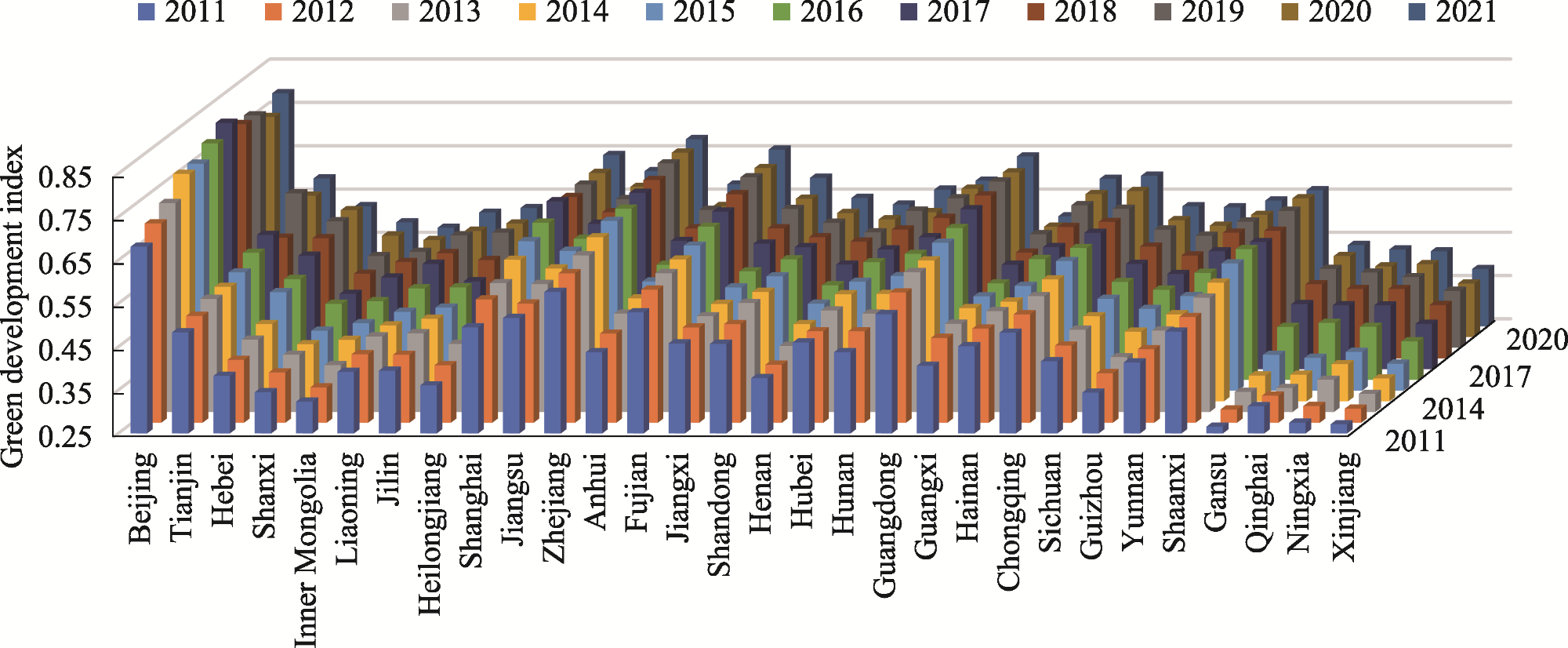
Figure 1 Green development index chart
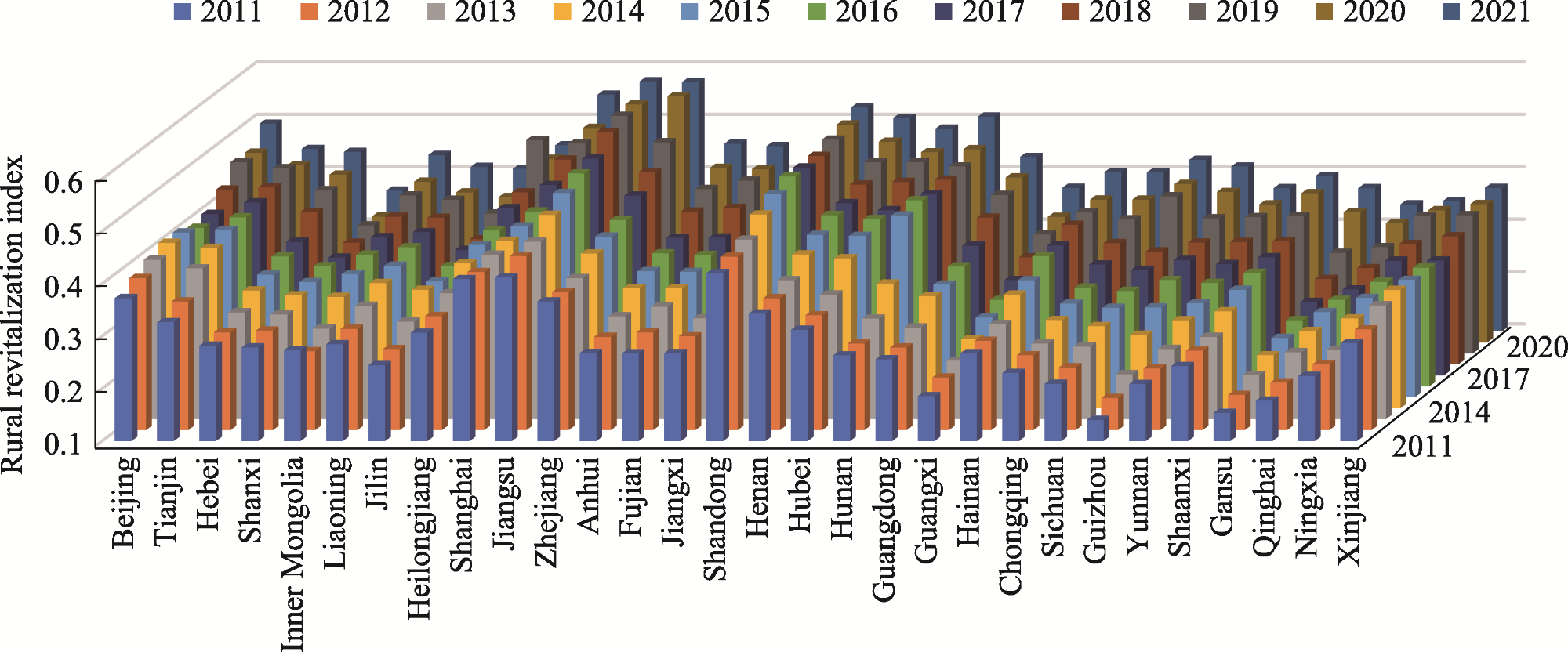
Figure 2 Rural revitalization index chart
Temporally, three characteristics can be observed: First, the green development level of various regions of China has risen annually, particularly around 2012 and 2015. These years marked the introduction of eco-environmental construction, and the new development philosophy of innovative, coordinated, green, open and shared development. During these periods, some provinces experienced significant increases in their green development levels. Second, rural revitalization overall has been rising, with fluctuating growth in some areas from 2011 to 2016. Influenced by the “Rural Revitalization Strategy”, a significant overall increase has been observed since 2017. Third, following the 2018 proposition of “boosting rural revitalization through green development,” most regions reached their peak in green development and rural revitalization in 2019. A slight decline was observed in 2020 due to the COVID-19, followed by a rebound in 2021. The green development and rural revitalization indices were higher in 2020 and 2021 than those before 2018, demonstrating significant effectiveness of green development in leading rural revitalization.
Regionally, in terms of green development levels, North and East China have higher green development levels due to their geographical advantages and economic foundations. Northeast and South Central China have moderate levels. Meanwhile, provinces in Southwest China, due to environmental advantages, have developed better. In contrast, Qinghai, Gansu, Ningxia, and Xinjiang, located in the northwest of China, have significantly lower green development levels due to harsh environments, weak development foundations, and greater developmental challenges. Next, in terms of rural revitalization, North, East, Northeast, and South Central China have generally higher rural revitalization levels as they are China’s main grain-producing areas with high levels of mechanization and superior natural geographical conditions. The differences between these regions are not significant. Southwest and Northwest China, characterized by mountain basins and desert arid areas with poor natural geographical conditions, lag behind. Except for Inner Mongolia, which has vast grasslands and open terrain, the remaining provinces in these regions have a significant developmental gap compared to other regions.

4.1.2 Spatial distribution characteristics

Utilizing the rural revitalization development index values of 30 provinces from 2011 to 2021, the global Moran’s I was calculated. As shown in Table 3, the global Moran’s I for the rural revitalization index is consistently greater than 0.2, while the P-value indicates that the Moran’s I is significant at the 99% confidence level. Thus, rural revitalization exhibits significant spatial positive correlation, indicating agglomeration.
Table 3 Rural revitalization global Moran’s I values
Year 2011 2012 2013 2014 2015 2016 2017 2018 2019 2020 2021
Moran’s I 0.385 0.377 0.380 0.340 0.282 0.246 0.286 0.330 0.290 0.319 0.324
P-value <0.001 <0.001 <0.001 <0.001 <0.001 0.001 <0.001 <0.001 <0.001 <0.001 <0.001

4.2 Spatial spillover effects

4.2.1 Analysis of results

Table 4 presents the linear and spatial regression results for the panel data of 30 provinces from 2011 to 2021. Columns I and II reports the results for ordinary least squares regressions, while columns III, IV, and V report the results for spatial Durbin model regressions. Column I shows that the regression coefficient for green development (Gre) is positive and significant at the 10% level, indicating that green development promotes rural revitalization (Rur). After introducing control variables, the regression coefficient for green development in column II remains significant at the 10% level and the sign of the coefficient does not change.
Table 4 Baseline regression results
Variables Ordinary least squares regressions Spatial Durbin model regressions
I II III IV V
L.Rur 0.914167***
(27.23)
Gre 0.5858161*
(1.90)
0.5707575*
(1.92)
0.5664907***
(6.00)
0.627408***
(6.56)
0.1451696**
(2.35)
W*Gre 0.9706973***
(4.03)
1.105201***
(4.15)
0.2628814*
(1.71)
ρ 0.1893467**
(1.97)
0.1850306*
(1.69)
0.2175777***
(2.67)
Controls No Yes Yes Yes Yes
Province Yes Yes Yes Yes Yes
Year Yes Yes Yes Yes Yes
R2 0.8254 0.8505 0.5835 0.5238 0.9365
Observation 330 330 330 330 330

Note: * indicates P<0.1; ** indicates P<0.05; *** indicates P<0.01. The same below.

To analyze the spatial spillover effect of green development on rural revitalization, this study performs a spatial Durbin model regression based on an economic-geographic weight matrix. The results from column III show that both the regression and spatial regression coefficients for green development are positive and significant at the 1% level. The spatial autocorrelation coefficient for rural revitalization is significant at the 5% level and positive, indicating a strong spatial spillover effect of green development on rural revitalization.

4.2.2 Decomposition effect analysis

To further delineate the magnitude and direction of the spatial spillover effects of various influencing factors, this study draws on LeSage’s (2010) study to decompose the impacts of core explanatory and control variables on the dependent variable into direct, indirect, and total effects, as shown in Table 5.
Table 5 Direct effects, indirect effects, and total effects results
Variables Direct effects Indirect effects Total effects
Gre 0.6033026***
(6.35)
1.286777***
(4.33)
1.890079***
(5.99)
Rgdp 0.0662152**
(2.47)
0.0714881
(0.90)
0.1377033
(1.64)
Gov -0.175383***
(-4.22)
-0.6303997***
(-3.65)
-0.8057827***
(-4.29)
Indus -0.1360138***
(-3.54)
-0.2772718**
(-2.29)
-0.4132856***
(-2.89)
Tra 0.0285738
(0.43)
-0.2928374
(-1.42)
-0.2642636
(-1.22)
lnInnov 0.0122342
(0.86)
-0.0262611
(-0.50)
-0.0140269
(-0.24)
lnEnv 0.0241186
(1.33)
-0.0237697
(-0.40)
0.0003489
(0.01)
The direct, indirect, and total effects of the core explanatory variable, the level of green development, are all significantly positive at the 1% level. Thus, green development promotes the revitalization of rural areas both locally and in adjacent areas, with a more pronounced effect on neighboring areas. This may be because the most direct change in green development is improving the environment. Such an improvement is systemic, benefiting not just the local area but also leading to the agglomeration effect when green development is pursued in various regions, thereby intensifying the spatial spillover effect.

4.2.3 The spatial spillover effect of rural revitalization on different levels of green development

The aforementioned spatial Durbin model is a commonly used model in the literature. This model not only confirms the significant promoting effect of green development on the rural revitalization level but also demonstrates the existence of spatial spillover effects of green development on rural revitalization. However, this model considers only a single spatial dependency mechanism. As China has a vast geographical expanse, the green development levels differ across different regions. Therefore, we need to examine whether the spatial spillover effects of rural revitalization differ under different green development levels. A two-regime spatial Durbin model can be used, it is possible to categorize the green development levels in different regions. This categorization is employed to capture the regional heterogeneity, enabling a more accurate analysis of the spatial spillover effects of rural revitalization under different green development levels. This study employs MATLAB for two-regime spatial Durbin model regression, with the results shown in Table 6.
Table 6 Two-regime spatial durbin model regression results
Variables Results
Gre 0.463072***
(5.52)
W*Gre 0.119709**
(2.39)
ρ1 0.522285***
(3.93)
ρ2 0.069952
(0.61)
ρ1-ρ2 0.4523**
(2.36)
Controls YES
Province YES
Year YES
R2 0.9544
Observation 330
First, with control variables, the coefficients for green development and its spatial regression are significant at the 1% level, signifying that green development significantly promotes rural revitalization. Second, Rho1, significantly positive at the 1% level with a value of 0.522285, indicates that areas with higher levels of green development exhibit more pronounced rural revitalization and stronger spillover effects. In contrast, Rho2 is not significantly positive and only equals 0.069952. This implies significant differences between areas with higher levels of green development and other regions.

4.2.4 Robustness test and endogenous problem

First, differences in models, data, and assumptions could yield different results. Considering the potential bidirectional causality between green development and rural revitalization. Specifically, advancing green development can promote rural revitalization and vice versa. However, this can cause endogeneity in the model, making parameter estimates inaccurate and affecting analysis results. Therefore, we perform robustness tests and address endogeneity.
(1) Robustness test
First, we change the weight matrix for robustness tests, recalculating the spatial Durbin model using an economic matrix. As indicated in Column IV of Table 4, under the economic matrix, the regression coefficient of green development and its spatial regression coefficient remain significantly positive. The spatial autoregression coefficient of rural revitalization has not changed significantly. This supports the robustness of our results.
(2) Endogenous problem
First, the study initially adopts a two-way fixed effects model for time and individuals, which alleviates endogeneity to some extent. Second, the dynamic spatial Durbin model is used for regression, introducing lagged dependent variables as explanatory variables. This approach addresses endogeneity issues, avoiding correlations between dependent and independent variables. The results in Column V of Table 4 show that the regression coefficient of green development and its spatial regression coefficient remain significant and unchanged compared to the static model. The spatial autoregression coefficient of rural revitalization and regression coefficient of the lagged dependent variable are both significantly positive, validating the dynamic spatial Durbin model results. After addressing endogeneity, the core explanatory variable, green development, still promotes rural revitalization in both the local and neighboring regions.

4.3 Spatial spillover network and identification of key nodes in the impact of green development on rural revitalization

The two-regime spatial Durbin model results in the previous subsection also demonstrated that areas with higher green development levels within a region had a more pronounced positive impact on the rural revitalization levels of surrounding areas. Therefore, as the process of green development and rural revitalization progresses, the development of key nodal provinces becomes particularly important. Here, we construct a spillover network through the decomposition matrix of spatial spillover effects and analyze. Finally, we employ complex network methods to identify key provincial nodes.

4.3.1 Network characteristics analysis

(1) Absolute spillover analysis
Based on complex network analysis methods, this study uses the spatial spillover effect matrix of green development on rural revitalization as the base data and employs ArcGIS to create a spatial spillover network of green development’s impact on rural revitalization across 30 provinces. This yields Figure 3 The direct impact effects are represented by the size of nodes, reflecting the direct impact values of green development on rural revitalization within each province. The thickness of the lines corresponds to the magnitude of spillover effects, while the distribution of spillover effects corresponds to the distribution of lines. Then, the network in Fig 3 is divided into four types based on threshold values of 20%, 40%, 60%, and 80% of the weights, resulting in Figure 4.
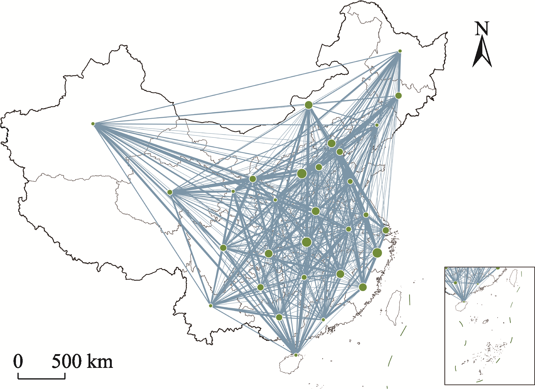
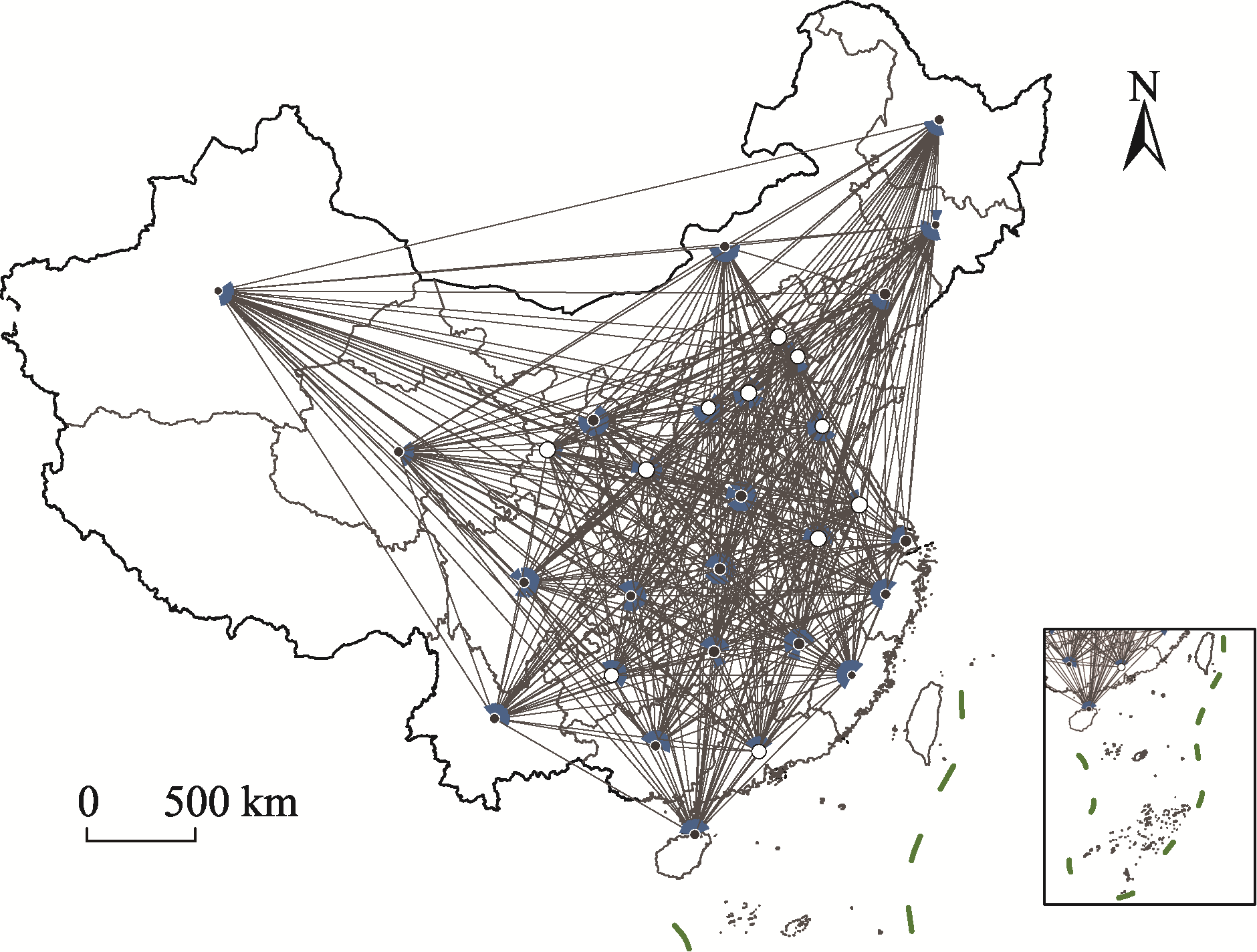
Figure 3 Spatial spillover network of green development on rural revitalization
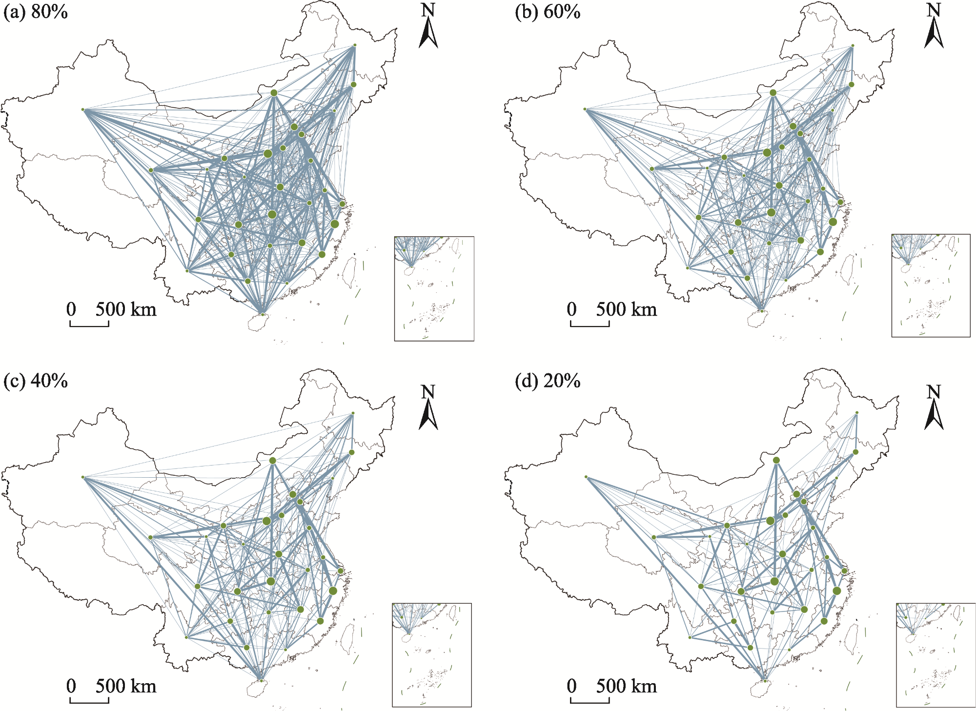
Figure 4 20%, 40%, 60% and 80% network split results
Figure 3 shows that provinces such as Anhui, Hebei, Shanxi, Jiangsu, Tianjin and Henan have a greater spillover impact of green development on rural revitalization in neighboring provinces. Meanwhile, provinces like Xinjiang, Heilongjiang, Jilin, Fujian, Yunnan, and Liaoning have a lower spillover impact.
As depicted in Figure 4, the network aligns with China's six major geographical divisions: North, Northeast, East, South Central, Southwest, and Northwest China. In North China, Hebei and Tianjin have higher centrality. In Northeast China, Liaoning has higher centrality. In East China, Anhui and Jiangsu have higher centrality. In South Central China, Hunan and Guangdong have higher centrality. In Southwest China, Guizhou and Sichuan have higher centrality. Finally, in Northwest China, Shaanxi and Gansu have higher centrality.
(2) Relative spillover analysis
Focusing solely on the absolute weights of nodes does not precisely define their overall position in the network and their relationship with other provinces. Therefore, we use NSIi and LSΓij to measure the relative weights of nodes. Based on the data of NSIi and LSΓij, a directional network of the spatial spillover of green development on rural revitalization is illustrated in Figure 5. The figure, the size of a node corresponds to the value of NSIi, with white and black-and siphon-type provinces, indicated by arrows for the spillover or siphon direction.
Figure 5 Direction-based green development’s spatial overflow network for rural revitalization
The node properties in Figure 5 reveal 13 spillover-type provinces: Beijing, Hebei, Tianjin, and Shanxi in North China; Jiangsu, Anhui, and Shandong in East China; Guangdong, Hunan, and Henan in South Central China; Guizhou in Southwest China; and Shaanxi and Gansu in Northwest China. Meanwhile, we have 17 siphon-type provinces, including Xinjiang, Jilin, and Fujian.
The direction of spillover or siphon in Figure 5 show that provinces such as Beijing, Jiangsu, Tianjin, Gansu, Shanghai, Anhui, Shaanxi, Hebei, Guangdong, and Shandong, have a spillover effect on more than 20 provinces. Meanwhile, Inner Mongolia, Fujian, Heilongjiang, Guangxi, Yunnan, Ningxia, Sichuan, Hainan, Jilin, and Xinjiang have a siphon effect on more than 20 provinces. Here, Beijing is a full-spillover province and Xinjiang is a full-siphon province.

4.3.2 Identification of key nodes

Drawing on extant research, internal and external factors were selected to identify key nodes. Internal factors were further divided into absolute spillover and relative spillover strength. Table 7 lists the details. The Entropy Method was used to measure the aforementioned indicators. Finally, based on China’s geographical divisions, the key provinces for the spillover effect of green development on rural revitalization were ultimately identified, as shown in Table 8.
Table 7 Relevant indicator data identified by important node provinces
Province Internal factors External factors Province Internal factors External factors
Spill strength Green development Spill strength Green development
Absolute Relative Average Absolute Relative Average
Beijing 1.5149 29 0.7649 Henan 1.5160 14 0.4630
Tianjin 1.5613 27 0.5396 Hubei 1.4967 13 0.5156
Hebei 1.7166 22 0.4760 Hunan 1.3877 19 0.5303
Shanxi 1.6536 16 0.4177 Guangdong 1.0732 21 0.5972
Inner Mongolia 1.1267 9 0.4182 Guangxi 1.1811 6 0.4745
Liaoning 1.0675 15 0.4588 Hainan 1.0896 2 0.5217
Jilin 0.9582 1 0.4601 Chongqing 1.1923 11 0.5475
Heilongjiang 0.9517 7 0.4503 Sichuan 1.3246 3 0.4765
Shanghai 1.1897 25 0.5932 Guizhou 1.3736 17 0.4446
Jiangsu 1.5734 28 0.5696 Yunnan 1.0455 5 0.4877
Zhejiang 1.4358 18 0.6413 Shaanxi 1.4229 23 0.5366
Anhui 1.7452 24 0.5155 Gansu 1.4094 26 0.3623
Fujian 0.9908 8 0.6009 Qinghai 1.1554 10 0.3656
Jiangxi 1.4444 12 0.5170 Ningxia 1.3666 4 0.3634
Shandong 1.4626 20 0.5150 Xinjiang 0.5408 0 0.3331
Table 8 Ranking of important node provinces in each region
Rank North China Northeast China East China South Central China Southwest China Northwest China
1 Beijing Liaoning Jiangsu Guangdong Guizhou Shaanxi
2 Tianjin Heilongjiang Shanghai Hunan Chongqing Gansu
3 Hebei Jilin Anhui Hubei Yunnan Qinghai
4 Shanxi Zhejiang Henan Sichuan Ningxia
5 Inner Mongolia Shandong Guangxi Xinjiang
6 Jiangxi Hainan
7 Fujian
Although Hebei and Shanxi have higher absolute spillover values, their relative spillover is limited. Further, their green development level is significantly different from that of Beijing. Therefore, Beijing is the key province for development in North China. Similarly, Guangdong is chosen for South Central China and Shaanxi for Northwest China. In Northeast China, the three provinces have similar absolute spillover values and green development levels, and are all siphon-type provinces. However, Liaoning stands out with its relative spillover, making it the key province for development in Northeast China. In East China, Jiangsu, compared to Shanghai, has a more evident absolute spillover and a higher green development level than Anhui, making it the key province for development. Among the four provinces in Southwest China, although Sichuan, Chongqing, and Yunnan have higher green development levels, they are all siphon-type provinces with limited relative spillover. Guizhou, with the highest absolute spillover value, a higher relative spillover, and being a spillover-type province, is the key province for development in Southwest China.

5 Discussion

This study reveals the spatiotemporal spillover effects and network characteristics of green development on rural revitalization through spatial econometric and complex network methodologies. We discuss our main findings below:
First, the spatial spillover effects of green development exhibit an “east-high, west-low” and “core-periphery” distribution pattern. Eastern coastal provinces, with their economic foundations and policy advantages, act as “core nodes” radiating green development. Meanwhile, northwestern regions, constrained by ecological fragility and resource limitations, predominantly remain “peripheral receivers”. While these findings align with Han and Gong’s (2025) “gradient diffusion theory of green economy”, they further highlight how regional heterogeneity modulates spillover pathways: High green development regions generate positive spillovers via technological diffusion and factor agglomeration, whereas low green development regions may exacerbate developmental imbalances through resource siphoning. Overcoming the “Matthew Effect” through policy interventions is pivotal for future regional synergy.
Second, some pivotal provinces serve dual roles as “engines” and “hubs” in the spillover network. For instance, Beijing influences neighboring provinces through policy innovation and capital exports, whereas Jiangsu drives green technological diffusion across the Yangtze River Delta via industrial transformation. This resonates with Chen et al.’s (2022) “global city network” theory. However, the nodal influence in rural revitalization hinges more on localized factors (e.g., agricultural modernization or ecological endowments) rather than sheer economic scale. Future research should disentangle differentiated pathways between “policy-driven” and “market-spontaneous” nodes.
Third, we identify some policy-practice paradoxes. Although green development significantly promotes rural revitalization, government intervention and industrial structure have negative effects. Thus, overreliance on administrative measures or reckless tertiary sector expansion may suppress endogenous rural dynamism. This corroborates with Cui and Wang’s (2024) warnings about “state-dominated green transition risks”, emphasizing the need to balance “top-down design” with “bottom-up innovation” to avoid homogenized governance.
Finally, this work has some limitations: First, although this study controlled for potential interferences from intra-provincial development disparities through the economic-geographical nested matrix and two-regime spatial Durbin model, a refined analysis at municipal and county scales remains unexplored due to data availability constraints. Future research can incorporate emerging data sources such as nighttime light and enterprise pollution emission data to further elucidate the cross-scale interaction mechanisms between green development and rural revitalization. Second, our findings may be constrained by the design of the indicator systems for green development and rural revitalization. Although split-sample testing and dynamic model validation have been employed to strengthen the robustness of conclusions, future research can explore nonlinear indicator synthesis methodologies (e.g., integrating Multi-Criteria Decision Making with machine learning) to enhance measurement objectivity. Finally, synergistic thresholds between green development and rural revitalization remain unquantified. Threshold models may clarify the critical conditions for policy optimization.

6 Conclusions and recommendations

6.1 Conclusions

This study utilized provincial panel data from 2011 to 2021, and employed the composite weighting method to measure the comprehensive index of green development and rural revitalization. It then analyzed the spatiotemporal evolution characteristics and influencing factors of green development on rural revitalization using the spatial Durbin model. Next, the two-regime spatial Durbin model was used to examine the impact of regional differences in green development on rural revitalization. Finally, key provinces were identified using complex network methods. Our main conclusions were as follows: 1) Both green development and rural revitalization levels in China rose annually, peaking in 2019. Key growth spurts occurred in 2012, 2015, and 2018 for green development, and 2018 for rural revitalization. 2) Green development boosted rural revitalization with spatial spillover effects. Economic growth, technological innovation, and infrastructure enhanced outcomes, while excessive government intervention or industrial expansion hindered progress. 3) High green development regions (eastern provinces) exhibit stronger spillover effects. In particular, northwestern provinces lag due to ecological and resource constraints. 4) Core nodes driving rural revitalization include Beijing (North), Liaoning (Northeast), Jiangsu (East), Guangdong (South Central), Guizhou (Southwest), and Shaanxi (Northwest).

6.2 Recommendations

First, policymakers should strengthen green policies, prioritizing investments in clean energy, green technology, and sustainable agriculture to amplify the spillover effects. Second, targeted infrastructure should be provided. Efforts should focus on upgrading rural transport, digital networks, and talent programs to balance urban-rural development and stimulate innovation. Finally, regional synergy should be leveraged by fostering collaboration between underdeveloped provinces and key nodes to mitigate disparities and share resources.
[1]
Chen Z, Sarkar A, Rahman A, et al. 2022. Exploring the drivers of green agricultural development (GAD) in China: A spatial association network structure approaches. Land Use Policy, 112: 105827. DOI: 10.1016/j.landusepol.2021.105827.

[2]
Cui X L, Wang R R. 2024. Spatial correlation network characteristics and influencing factors of coordinated development of low-carbon, pollution reduction, ecological expansion and growth in China. Research of Environmental Science, 37(7): 1446-1457. (in Chinese)

[3]
Duan Y F. 2019. Value implications and practical directions of green development from the perspective of rural revitalization. Chongqing Social Sciences, (12): 6-13. (in Chinese)

[4]
Fu J H, Xue J X. 2024. Digital village construction, rural human capital and agricultural green development. Survey World, (1): 15-25. (in Chinese)

[5]
Han H B, Gong Y S. 2025. Spatial spillover effects of digital village construction on agricultural carbon emissions. Journal of Agricultural Engineering, 41(1): 298-307. (in Chinese)

[6]
Hu X P, Yue D. 2022. Has environmental regulation promoted agricultural total factor productivity? Jianghan Forum, (11): 42-51. (in Chinese)

[7]
Jin G, Shen K R. 2018. Beggar-thy-neighbor or partner? Environmental regulation enforcement interaction and urban productivity growth. Management World, 34(12): 43-55. (in Chinese)

[8]
LeSage J P, Fischer M M. 2010. Spatial econometric methods for modeling origin-destination flows. In: Fischer MM, GetisA (eds.). Handbook of applied spatial analysis. Berlin, Germany: Springer: 409-433.

[9]
Li F R, Yan Y. 2023. An economic analysis of rural green development in China: Based on the theoretical interpretation of pollution governance subject alienation. Economic Issues, (8): 7-16. (in Chinese)

[10]
Li X X, Pan J C. 2011. Compilation of China’s green development index: A summary of the 2010 provincial comparative report. Economic Research Reference, (2): 36-64. (in Chinese)

[11]
Li Y X, Yu F W. 2024. The internal logic, key tasks and practical paths of rural ecological revitalization under the “dual-carbon” goals. Gansu Social Sciences, (5): 206-213. (in Chinese)

[12]
Limtanakool N, Dijst M. 2009. Developments in the Dutch urban system on the basis of flows. Regional Studies, 43: 179-196.

DOI

[13]
Limtanakool N, Dijst M, Schwanen T. 2007. A theoretical framework and methodology for characterizing national urban systems on the basis of flows of people: Empirical evidence for France and Germany. Urban Studies, 44: 2123-2145.

DOI

[14]
Mao J H. 2021. Improved methodology and empirical study on rural revitalization evaluation index system. Journal of Lanzhou University (Social Sciences), 49(3): 47-58. (in Chinese)

[15]
Mol A P J. 2000. Ecological modernization:Industrial transformations and environmental reform. In: RedcliftM, WoodgateG (eds.). The international handbook of environmental sociology. Cheltenham, UK: Edward Elgar: 138-149.

[16]
Rapport D J, Friend T. 1979. Towards a comprehensive framework for environmental statistics:A stress-response approach. Ottawa, Canada: Statistics Canada.

[17]
Suo L M, Leng X Z. 2024. The“adaptive nesting” logic of regional environmental collaborative governance in China: An analysis based on social-ecological systems framework. Theory and Reform, (5): 109-128. (in Chinese)

[18]
Tang Y X, Ma J L, Liu L H. 2024. Coordination relationship and influencing factors between green development and rural revitalization in Sichuan-Guizhou regions. Bulletin of Soil and Water Conservation, 44(4): 277-288. (in Chinese)

[19]
Tao J X, Huang Y R. 2005. Research on green GDP accounting system. Science & Technology Progress and Policy, (10): 25-27. (in Chinese)

[20]
Tortosa L, Yeghikyan G, Vicent J F. 2021. An algorithm for ranking the nodes of multiplex networks with data based on the PageRank concept. Applied Mathematics and Computation, 392: 125676. DOI: 10.1016/j.amc.2020.125676.

[21]
Wan J, Li S Q, Zhang Q. 2022. Measurement, pattern and logic of rural revitalization in China. Guizhou Social Sciences, (3): 143-152. (in Chinese)

[22]
Wang S X, Hu Y Y, Tang P P. 2021. Construction of long-term dynamic mechanisms for coordinated advancement of rural revitalization and green development in contiguous poverty-stricken areas. Contemporary Economic Management, 43(4): 33-38. (in Chinese)

[23]
Wang Z, Li T, Huang W J. 2023. Connotation, components and research framework of urban-rural logistics network from a spatial perspective. Scientia Geographica Sinica, 43(1): 82-91. (in Chinese)

[24]
Wen C H, Zhang J Y, Li W Y. 2023. Integrated green development in Chengdu-Kunming-Chongqing regions: Logical rationale, practical dilemmas and implementation pathways. Chongqing Social Sciences, (8): 122-132. (in Chinese)

[25]
Xie T T, Feng M J. 2023. Green finance empowering rural revitalization: With discussion on the mediating effect of agricultural eco-efficiency. Price: Theory & Practice, (6): 174-178, 212. (in Chinese)

[26]
Xiong M, Li W, Teo B S X, et al. 2022. Can China’s digital inclusive finance alleviate rural poverty? An empirical analysis from the perspective of regional economic development and an income gap. Sustainability, 14(24): 16984. DOI: 10.3390/su142416984.

[27]
Yan X, Zou C, Qian X Y. 2023. Spatial correlation network evolution and driving factors of intercity eco-green development in the Yangtze River Delta. Journal of Hohai University (Philosophy and Social Sciences), 25(6): 120-131. (in Chinese)

[28]
Zhong S, Li X, Zhang Y L. 2022. Rural revitalization under green development: Connotation interpretation, realization mechanisms and implementation paths. Chinese Landscape Architecture, 38(6): 35-39. (in Chinese)

[29]
Zhou H H, Gu G F, Ren H M. 2024. Impact of urban network status on economic growth in China from a multi-source data perspective. Economic Geography, 44(10): 55-65. (in Chinese)

Outlines

/