
Journal of Resources and Ecology >
The Effects and Mechanisms of Rural Digitalization and Agricultural Carbon Reduction
|
HUANG Longjunjiang, E-mail: huanglongjunjiang@stu.zuel.edu.cn |
Received date: 2025-10-29
Accepted date: 2025-12-30
Online published: 2026-02-02
Supported by
The Key Project of the Key Research Base for Philosophy and Social Sciences in Jiangxi Province(23ZXSKJD07)
Investigating the impact of rural digitalization on agricultural carbon emissions contributes to achieving carbon neutrality goals and facilitates the green transformation of agriculture with enhanced efficiency. Based on panel data from 31 provincial-level regions in China spanning 2005 to 2022, this study employs a dynamic panel model to analyze the influence of rural digitalization on agricultural carbon emission intensity. Heterogeneity analysis, mechanism testing, and spatial effect examination are also conducted. The main findings are fourfold. (1) Rural digitalization effectively promotes the reduction of agricultural carbon emissions. (2) Heterogeneity analysis revealed that the effect of rural digitalization on lowering agricultural carbon emission intensity is particularly significant in production-marketing balanced regions. (3) The carbon emission reduction effect of rural digitalization is primarily realized through the scaling of agricultural operations, the accumulation of human capital, and the improvement of total factor productivity. (4) A positive spatial correlation exists in the agricultural carbon emission intensity across provinces, and the inhibitory effect of rural digitalization on agricultural carbon emission intensity exhibits spatial spillover effects. Therefore, to accelerate rural digitalization and advance agricultural carbon emission reduction, it will be essential to promote the scaling of agricultural operations, guide farmers in adopting advanced technologies, and enhance their ability to utilize digital tools.
HUANG Longjunjiang , LI Lishan , LIU Xiaojin . The Effects and Mechanisms of Rural Digitalization and Agricultural Carbon Reduction[J]. Journal of Resources and Ecology, 2026 , 17(1) : 275 -290 . DOI: 10.5814/j.issn.1674-764x.2026.01.022
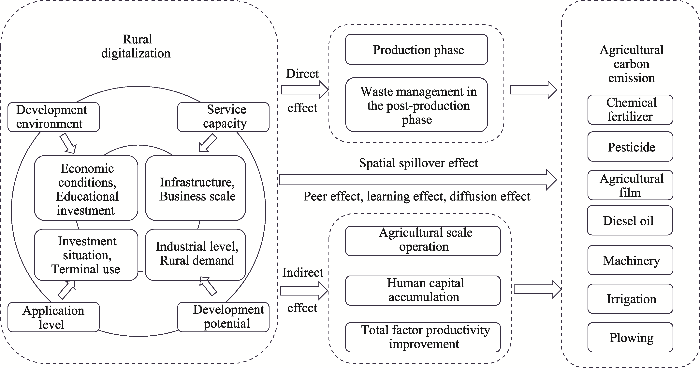
Figure 1 Theoretical analysis framework |
Table 1 Rural digitalization level index system |
| Primary indicator | Secondary indicator | Indicator name and unit | Property | Indicator weight |
|---|---|---|---|---|
| Development environment | Economic condition | Per capita actual output value of agriculture, forestry, animal husbandry and fishery (104 yuan person-1) | + | 0.030 |
| Per capita disposable income of rural residents (104 yuan person-1) | + | 0.038 | ||
| Comparison of income levels between urban and rural residents (rural residents = 1) | - | 0.008 | ||
| Length of rural postal delivery lines (km km-2) | + | 0.061 | ||
| Educational investment | Rural residents’ consumption expenditure on education and entertainment (yuan person-1) | + | 0.029 | |
| Proportion of rural residents’ consumption expenditure on education and entertainment (%) | + | 0.010 | ||
| Service capacity | Infrastructure | Long-distance automatic switchboard capacity (road terminals (104 persons) -1) | + | 0.049 |
| Local telephone office switchboard capacity (doors person-1) | + | 0.051 | ||
| Mobile telephone switchboard capacity (households person-1) | + | 0.032 | ||
| Length of long-distance optical cable line (km km-2) | + | 0.037 | ||
| Business scale | Per capita business volume of the telecommunications industry (104 yuan person-1) | + | 0.090 | |
| Number of fixed telephone users per capita (per person) | + | 0.032 | ||
| Number of mobile phone users per capita (per person) | + | 0.021 | ||
| Per capita mobile phone call time (104 minutes person-1) | + | 0.013 | ||
| Per capita business volume of mobile text message (104 messages person-1) | + | 0.052 | ||
| Average number of Internet users per capita (per person) | + | 0.028 | ||
| Application level | Investment situation | Rural residents’ consumption expenditure on transportation and communication (yuan person-1) | + | 0.040 |
| Proportion of rural residents’ consumption expenditure on transportation and communication (%) | + | 0.010 | ||
| Terminal use | Comprehensive population coverage rate of rural radio programs (%) | + | 0.005 | |
| Comprehensive population coverage rate of rural TV programs (%) | + | 0.005 | ||
| Popularity of color TV in rural areas (units/100 households) | + | 0.008 | ||
| Rural mobile phone popularity (departments/100 households) | + | 0.015 | ||
| Computer popularity in rural areas (units/100 households) | + | 0.055 | ||
| Number of Internet broadband access ports per capita (number per person) | + | 0.051 | ||
| Proportion of rural broadband access users (%) | + | 0.023 | ||
| Proportion of administrative villages with Internet broadband services (%) | + | 0.003 | ||
| Development potential | Industrial level | Proportion of main business income of the telecommunications industry to GDP (%) | + | 0.031 |
| Number of employees as a percentage of total employed persons (%) | + | 0.066 | ||
| Proportion of related investment to total social fixed asset investment (%) | + | 0.032 | ||
| Proportion of tax revenue from the digital information industry (%) | + | 0.033 | ||
| Rural demand | Added value of the primary industry accounts as a proportion of regional GDP (%) | + | 0.025 | |
| Proportion of rural population to total population (%) | + | 0.017 |
Table 2 Measurement of agricultural total factor productivity indicators |
| Indicator type | Primary indicator | Secondary indicator | Indicator meaning |
|---|---|---|---|
| Input indicators | Land input | Land input | Total crop sown area (103 ha) |
| Labor input | Rural labor input | Number of employees in rural primary industry (104 persons) | |
| Other labor inputs | Number of employees in agriculture, forestry, animal husbandry and fishery in urban units (104 persons) | ||
| Capital input | Mechanical input | Total power of agricultural machinery (104 kW) | |
| Draught animal input | Year-end stock of large livestock (104 heads) | ||
| Fertilizer input | Agricultural chemical fertilizer application amount calculated by the purity conversion method (104 t) | ||
| Pesticide input | Pesticide usage (104 t) | ||
| Agricultural film input | Agricultural plastic film usage (104 t) | ||
| Resource input | Water resources input | Effective irrigated area (103 ha) | |
| Energy input | Rural electricity consumption (108 kWh) | ||
| Fuel input | Agricultural diesel consumption (104 t) | ||
| Output indicators | Expected output | Economic output | Actual total output value of agriculture, forestry, animal husbandry and fishery (108 yuan) |
Table 3 Descriptive statistics of the variables |
| Variable | Variable code | Sample size | Average | Standard deviation | Minimum | Maximum |
|---|---|---|---|---|---|---|
| Agricultural carbon intensity | ACI | 558 | 0.138 | 0.051 | 0.036 | 0.323 |
| Rural digitization level | RDL | 558 | 0.251 | 0.083 | 0.118 | 0.564 |
| Agricultural planting structure | APS | 558 | 0.654 | 0.136 | 0.328 | 0.971 |
| Agricultural industrial structure | AIS | 558 | 0.521 | 0.086 | 0.302 | 0.746 |
| Natural disaster impact | NDI | 558 | 0.182 | 0.145 | 0.000 | 0.936 |
| Urbanization level | UL | 558 | 0.554 | 0.147 | 0.209 | 0.896 |
| Industrialization level | IL | 558 | 0.360 | 0.102 | 0.068 | 0.536 |
| Openness level | OL | 558 | 0.288 | 0.345 | 0.008 | 1.721 |
| Land quality | LQ | 558 | 0.439 | 0.190 | 0.154 | 1.233 |
| Agricultural mechanization level | AML | 558 | 4.461 | 2.379 | 0.739 | 13.689 |
| Scale agricultural operation | SAO | 558 | 7.419 | 4.002 | 2.551 | 29.362 |
| Human capital accumulation | HCA | 558 | 7.543 | 0.860 | 3.804 | 9.877 |
| Agricultural total factor productivity | ATFP | 558 | 1.738 | 0.825 | 0.609 | 5.381 |
Table 4 Estimation results of rural digitalization level on agricultural carbon intensity |
| Variable | Model 1 OLS | Model 2 FE | Model 3 RE | Model 4 GMM | Model 5 GMM |
|---|---|---|---|---|---|
| RDL | -0.168*** | -0.082* | -0.078* | -0.105*** | -0.140*** |
| (0.043) | (0.042) | (0.044) | (0.012) | (0.016) | |
| APS | 0.055*** | -0.033 | 0.018 | 0.066*** | 0.037 |
| (0.013) | (0.023) | (0.021) | (0.012) | (0.041) | |
| AIS | 0.250*** | 0.013 | 0.047* | 0.058*** | 0.051*** |
| (0.017) | (0.026) | (0.026) | (0.010) | (0.013) | |
| NDI | 0.101*** | 0.012 | 0.023*** | -0.003 | -0.002 |
| (0.011) | (0.008) | (0.008) | (0.002) | (0.002) | |
| UL | -0.049** | -0.379*** | -0.307*** | -0.130*** | 0.038 |
| (0.024) | (0.028) | (0.028) | (0.016) | (0.023) | |
| IL | 0.132*** | -0.024 | 0.027 | -0.084*** | -0.038*** |
| (0.018) | (0.022) | (0.022) | (0.007) | (0.006) | |
| OL | 0.032*** | 0.016** | 0.027*** | 0.001 | 0.004** |
| (0.007) | (0.007) | (0.007) | (0.002) | (0.002) | |
| LQ | 0.062*** | -0.009 | 0.014 | 0.024*** | 0.026*** |
| (0.010) | (0.015) | (0.014) | (0.003) | (0.005) | |
| AML | -0.001 | 0.000 | -0.001 | -0.003*** | -0.003*** |
| (0.001) | (0.001) | (0.001) | (0.001) | (0.001) | |
| L. ACI | 0.629*** | 0.824*** | |||
| (0.029) | (0.030) | ||||
| Constant term | -0.059*** | 0.389*** | 0.267*** | 0.106*** | -0.001 |
| (0.017) | (0.031) | (0.029) | (0.014) | (0.032) | |
| R2 | 0.592 | 0.152 | 0.246 | ||
| AR (1) | 0.015 | 0.009 | |||
| AR (2) | 0.202 | 0.126 | |||
| Sargan test | 0.547 | 0.999 | |||
| N | 558 | 558 | 558 | 496 | 527 |
Note: ***, ** and * indicate significance at the statistical levels of 1%, 5% and 10%, respectively, and the values in parentheses are standard errors. The significance probability P-values were obtained using the Arellano-Bond and Sargan tests. The change in the sample size N is due to model specification rather than human modification. The same applies to the following tables. |
Table 5 Robustness test |
| Variable | Model 6 Replacing the explained variable | Model 7 Increasing the control variables | Model 8 Removing outlier provinces | Model 9 Eliminating outlier years | Model 10 Winsorization |
|---|---|---|---|---|---|
| RDL | -0.034*** | -0.133*** | -0.179*** | -0.137*** | -0.150*** |
| (0.005) | (0.014) | (0.020) | (0.017) | (0.016) | |
| Control variable | Yes | Yes | Yes | Yes | Yes |
| FSL | -0.100*** | ||||
| (0.028) | |||||
| L. ACI | 0.962*** | 0.802*** | 0.799*** | 0.791*** | 0.820*** |
| (0.015) | (0.040) | (0.055) | (0.019) | (0.035) | |
| Constant term | 0.002 | -0.014 | 0.070 | -0.020 | -0.009 |
| (0.005) | (0.043) | (0.071) | (0.016) | (0.021) | |
| AR (1) | 0.031 | 0.008 | 0.022 | 0.019 | 0.001 |
| AR (2) | 0.256 | 0.110 | 0.215 | 0.072 | 0.365 |
| Sargan test | 0.999 | 0.999 | 0.999 | 0.998 | 0.999 |
| N | 527 | 527 | 459 | 434 | 527 |
Table 6 Regression results based on regional heterogeneity analysis |
| Variable | Model 11 Main grain producing area | Model 12 Major grain sales area | Model 13 Production-sales balanced area |
|---|---|---|---|
| RDL | -0.147*** | -0.167*** | -0.116*** |
| (0.016) | (0.012) | (0.014) | |
| Whether it is in the major grain producing area * RDL | 0.000 | ||
| (0.031) | |||
| Whether it is in the major grain producing area | -0.005 | ||
| (0.019) | |||
| Whether it is in the major grain sales area * RDL | 0.046 | ||
| (0.037) | |||
| Whether it is in the major grain sales area | 0.002 | ||
| (0.016) | |||
| Whether it is in the production and sales balanced area * RDL | -0.065*** | ||
| (0.024) | |||
| Whether it is in the production and sales balanced area | 0.009 | ||
| (0.012) | |||
| Control variable | Yes | Yes | Yes |
| L. ACI | 0.804*** | 0.806*** | 0.804*** |
| (0.031) | (0.030) | (0.028) | |
| Constant term | -0.011 | -0.018 | -0.003 |
| (0.020) | (0.018) | (0.018) | |
| AR (1) | 0.010 | 0.009 | 0.009 |
| AR (2) | 0.108 | 0.109 | 0.107 |
| Sargan test | 0.762 | 0.748 | 0.791 |
| N | 527 | 527 | 527 |
Note: “Whether it is in the major grain producing area * RDL” is the interaction term between “Whether it is in the major grain producing area” and “RDL”, representing the product of the two variables. The same applies to the similar variables in the table. |
Table 7 Regression results based on mechanism studies |
| Variable | Model 14 Scale agricultural operation | Model 15 Human capital accumulation | Model 16 Agricultural total factor productivity |
|---|---|---|---|
| RDL | 8.347*** | 1.473*** | 3.749*** |
| (0.524) | (0.313) | (0.491) | |
| Control variable | Yes | Yes | Yes |
| L. SAO | 0.860*** | ||
| (0.015) | |||
| L. HCA | 0.533*** | ||
| (0.039) | |||
| L. ATFP | 0.914*** | ||
| (0.020) | |||
| Constant term | 0.876* | 1.574*** | -0.471 |
| (0.513) | (0.475) | (0.298) | |
| AR (1) | 0.005 | 0.009 | 0.014 |
| AR (2) | 0.129 | 0. 698 | 0.240 |
| Sargan test | 0.651 | 0.588 | 0.695 |
| N | 527 | 527 | 527 |
Table 8 Global Moran’s I index table |
| Year | Moran’s I | Year | Moran’s I | Year | Moran’s I | Year | Moran’s I | Year | Moran’s I | Year | Moran’s I |
|---|---|---|---|---|---|---|---|---|---|---|---|
| 2005 | 0.190** | 2008 | 0.122* | 2011 | 0.151** | 2014 | 0.184** | 2017 | 0.246*** | 2020 | 0.330*** |
| 2006 | 0.179** | 2009 | 0.171** | 2012 | 0.200** | 2015 | 0.198** | 2018 | 0.265*** | 2021 | 0.399*** |
| 2007 | 0.189** | 2010 | 0.170** | 2013 | 0.192** | 2016 | 0.237*** | 2019 | 0.301*** | 2022 | 0.360*** |
Table 9 Test results of spatial econometric model selection |
| Test method | Statistical value | P-value |
|---|---|---|
| LM test, no spatial error | 294.551*** | <0.001 |
| Robust LM test, no spatial error | 98.633*** | <0.001 |
| LM test, no spatial lag | 196.053*** | <0.001 |
| Robust LM test, no spatial lag | 0.135 | 0.713 |
| Hausman | 52.080*** | <0.001 |
| LR Lag | 129.180*** | <0.001 |
| LR Err | 123.520*** | <0.001 |
| Wald Lag | 27.350*** | 0.001 |
| Wald Err | 23.770*** | 0.005 |
Table 10 Regression results and decomposition of the spatial Durbin model |
| Variable | Model 17 0-1 Adjacency matrix | Model 18 Economic distance weight matrix |
|---|---|---|
| RDL | -0.214*** | -0.249*** |
| (0.057) | (0.056) | |
| Control variable | Yes | Yes |
| Wx | -0.129 | -0.451*** |
| (0.097) | (0.150) | |
| ρ | -0.169*** | -0.169** |
| (0.061) | (0.082) | |
| σ²_e | 0.000*** | 0.000*** |
| (0.000) | (0.000) | |
| Direct effect | -0.209*** | -0.234*** |
| (0.060) | (0.059) | |
| Indirect effect | -0.081 | -0.361*** |
| (0.092) | (0.137) | |
| Total utility | -0.290*** | -0.595*** |
| (0.082) | (0.134) | |
| R2 | 0.157 | 0.208 |
| N | 558 | 558 |
| [1] |
|
| [2] |
|
| [3] |
|
| [4] |
|
| [5] |
|
| [6] |
|
| [7] |
|
| [8] |
|
| [9] |
|
| [10] |
|
| [11] |
|
| [12] |
|
| [13] |
|
| [14] |
|
| [15] |
|
| [16] |
|
| [17] |
|
| [18] |
|
| [19] |
|
| [20] |
|
| [21] |
|
| [22] |
|
| [23] |
|
| [24] |
|
| [25] |
|
| [26] |
|
| [27] |
|
| [28] |
|
| [29] |
|
| [30] |
|
| [31] |
|
| [32] |
|
| [33] |
|
| [34] |
|
| [35] |
|
| [36] |
|
| [37] |
|
| [38] |
|
| [39] |
|
| [40] |
|
| [41] |
|
| [42] |
|
| [43] |
|
| [44] |
|
| [45] |
|
| [46] |
|
| [47] |
|
| [48] |
|
| [49] |
|
| [50] |
|
| [51] |
|
/
| 〈 |
|
〉 |