
Journal of Resources and Ecology >
Regional Differences in the Driving Factors and Decoupling Relationships of Carbon Emissions in Inner Mongolia
|
SUN Baojun, E-mail: sunbaojun@126.com |
Received date: 2025-04-25
Accepted date: 2025-07-22
Online published: 2025-10-14
Supported by
The National Natural Science Foundation of China(71961022)
The Natural Science Foundation of Inner Mongolia Autonomous Region(2024MS07012)
The Fundamental Research Funds for the Central Universities of Inner Mongolia Autonomous Region(NCYWT23034)
The Fundamental Research Funds for the Central Universities of Inner Mongolia Autonomous Region(NCYWT23043)
The Inner Mongolia University of Finance and Economics 2025 High-Quality Research Achievements Cultivation Fund Project(GZCG24247)
The Inner Mongolia University of Finance and Economics 2025 High-Quality Research Achievements Cultivation Fund Project(GZCG2504)
The Special Research Project on the Five Major Tasks of Inner Mongolia Autonomous Region by Inner Mongolia University of Finance and Economics(NCXWD2419)
The Project of the Regional Digital Economy and Digital Governance Research Center of Inner Mongolia University of Finance and Economics(SZZL202401)
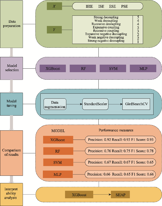
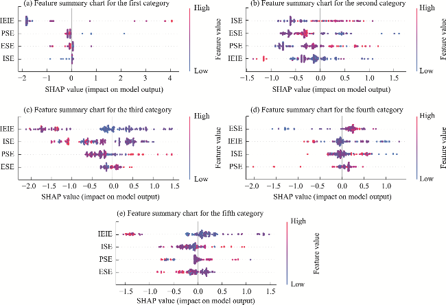
Within the framework of China's pursuit of green and low-carbon development, Inner Mongolia is characterized by significant carbon emissions, a substantial share of energy-intensive industries, and disparate development levels across its cities, so it faces substantial challenges in attaining the objectives of carbon peak and neutrality. Utilizing the Logarithmic Mean Divisia Index (LMDI) model, this study investigated the drivers and regional differences in carbon emissions. Drawing upon Tapio’s decoupling framework, the decoupling status between economic growth and carbon emissions among cities was analyzed in phases. We introduced the Extreme Gradient Boosting (XGBoost) machine learning algorithm to construct a classification model that correlates carbon emission drivers with decoupling states, elucidated by the Shapley Additive exPlanations (SHAP) interpretable model, and performed a spatial analysis of regional differences to assess the significance of industrial energy intensity for achieving strong decoupling in each prefecture-level city. The outcomes revealed two main results. (1) Spatially, regional differences in the influence of driving factors can be classified into four categories: energy intensity-dominant, double-effect negative driven, coexistence of positive and negative effects, and economic growth-driven. (2) Temporally, regional differences in the impact of industrial energy intensity on strong decoupling can be categorized into three types: overall positive, marked fluctuation, and stage stability. Consequently, tailoring emission reduction policies based on regional differences will be instrumental for expediting the achievement of the “dual carbon” targets.
Key words: LMDI model; Tapio decoupling analysis; XGBoost; SHAP; regional differences
SUN Baojun , LIANG Yuqing . Regional Differences in the Driving Factors and Decoupling Relationships of Carbon Emissions in Inner Mongolia[J]. Journal of Resources and Ecology, 2025 , 16(5) : 1327 -1342 . DOI: 10.5814/j.issn.1674-764x.2025.05.007
Table 1 Decoupling status and descriptions |
| Type | Decoupling status | ΔC | ΔG | Ɛ | Status description | Classification |
|---|---|---|---|---|---|---|
| Decoupling | Strong decoupling | $<$0 | $>$0 | $\left( -\infty,0 \right)$ | Carbon emissions decrease while the economy remains in a growth state, representing the most ideal scenario for urban development | 5 |
| Weak decoupling | $>$0 | $>$0 | $\left[ 0,0.8 \right]$ | Carbon emissions increase and the economy grows, but at a rate lower than the economic growth | 4 | |
| Recessive decoupling | $<$0 | $<$0 | $\left( 1.2,+\infty \right)$ | Carbon emissions decrease alongside an economic recession. | ||
| Coupling | Expansive coupling | $>$0 | $>$0 | $\left[ 0.8,1.2 \right]$ | Carbon emissions increase concurrently with economic growth, with the rates being comparable | 3 |
| Recessive coupling | $<$0 | $<$0 | $\left[ 0.8,1.2 \right]$ | Carbon emissions decrease while the economy also declines, with the rate of decrease being equivalent to the economic decline | ||
| Negative decoupling | Expansive negative decoupling | $>$0 | $>$0 | $\left( 1.2,+\infty \right)$ | Carbon emissions increase and the economy grows, with the growth rate exceeding that of the economy | 2 |
| Weak negative decoupling | $<$0 | $<$0 | $\left[ 0,0.8 \right]$ | Carbon emissions decrease while the economy declines, with the rate of decrease being less than the economic decline | ||
| Strong negative decoupling | $>$0 | $<$0 | $\left( -\infty,0 \right)$ | Carbon emissions increase alongside an economic recession, representing the least ideal scenario for urban development | 1 |
Figure 1 Technical roadmap for model selection |
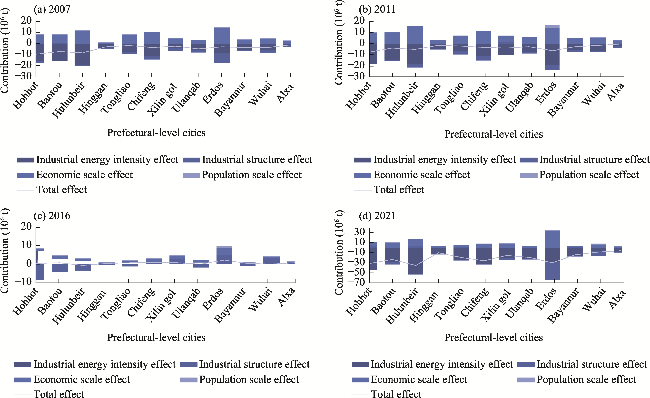
Figure 2 Effect analysis of various driving factors (10⁶ t) |
Table 2 LMDI decomposition results of carbon emissions for various cities and prefectures in Inner Mongolia in 2021(10⁶ t) |
| City | IEIE | ISE | ESE | PSE | TE |
|---|---|---|---|---|---|
| Hohhot | -43.639 | 4.041 | 7.206 | 0.890 | -31.503 |
| Baotou | -29.295 | -3.623 | 10.177 | 0.172 | -22.570 |
| Hulunbeir | -51.877 | 3.692 | 14.069 | -0.915 | -35.030 |
| Hinggan | -12.197 | 0.669 | 2.159 | -0.120 | -9.489 |
| Tongliao | -24.096 | 1.122 | 4.566 | -0.218 | -18.626 |
| Chifeng | -33.141 | 0.381 | 7.184 | -0.187 | -25.763 |
| Xilin Gol | -19.536 | -3.938 | 8.098 | 0.275 | -15.102 |
| Ulanqab | -22.058 | -0.164 | 4.609 | -0.892 | -18.504 |
| Erdos | -29.575 | -34.298 | 34.044 | 0.713 | -29.116 |
| Bayannur | -17.695 | 0.912 | 3.879 | -0.169 | -13.073 |
| Wuhai | -6.330 | -9.048 | 7.006 | 0.068 | -8.305 |
| Alxa | -7.209 | -2.161 | 2.953 | 0.167 | -6.250 |
Note: IEIE: Industry Energy Intensity Effect; ISE: Industry Structure Effect; ESE: Economic Scale Effect; PSE: Population Scale Effect; TE: Total Effect. The same below. |
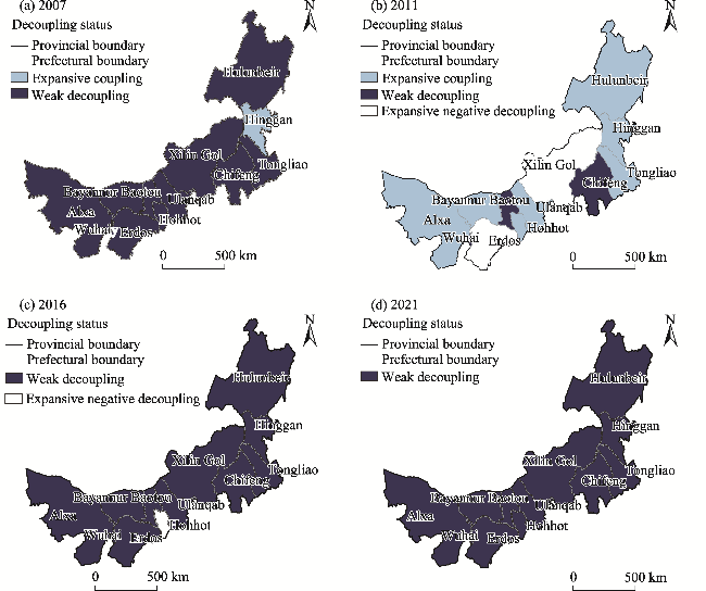
Table 3 Decoupling status of various cities in Inner Mongolia from 2007 to 2021 |
| Year | Hohhot | Baotou | Hulunbeir | Hinggan | Tongliao | Chifeng | Xilin Gol | Ulanqab | Erdos | Bayannur | Wuhai | Alxa |
|---|---|---|---|---|---|---|---|---|---|---|---|---|
| 2007 | WD | WD | WD | EC | WD | WD | WD | WD | WD | WD | WD | WD |
| 2008 | WD | WD | WD | WD | WD | WD | WD | WD | WD | WD | WD | WD |
| 2009 | WD | WD | WD | WD | WD | WD | WD | WD | WD | WD | WD | WD |
| 2010 | EC | EC | WD | EC | WD | WD | EC | END | EC | EC | WD | WD |
| 2011 | EC | WD | EC | EC | EC | WD | END | EC | END | EC | WD | EC |
| 2012 | SD | SD | SD | WD | SD | SD | WD | WD | WD | SD | SD | WD |
| 2013 | WD | SD | WD | WD | WD | WD | WD | WD | WD | WD | SD | WD |
| 2014 | WD | WD | WD | WD | END | WD | WD | WD | WD | WD | WD | WND |
| 2015 | SD | SD | SD | SD | SD | SD | SD | SD | SD | SD | WND | SD |
| 2016 | END | WD | WD | WD | WD | WD | WD | WD | WD | WD | WD | WD |
| 2017 | WD | WD | SD | WD | END | WD | SD | WD | SD | SD | WD | SD |
| 2018 | SND | SND | SND | SND | SND | SND | SND | SND | SND | SND | SND | SND |
| 2019 | WD | WD | WD | WD | WD | WD | WD | WD | WD | WD | WD | WD |
| 2020 | END | WD | SND | WD | END | WD | WD | WD | SND | SND | WD | WD |
| 2021 | WD | WD | WD | WD | WD | WD | WD | WD | WD | WD | WD | WD |
Note: SD, WD, RD, EC, RC, END, WND, and SND represent Strong decoupling, Weak decoupling, Recessive decoupling, Expansive coupling, Recessive coupling, Expansive negative decoupling, Weak negative decoupling, and Strong negative decoupling, respectively. |
Figure 3 Visualization of decoupling status |
Figure 4 SHAP category summary plots |
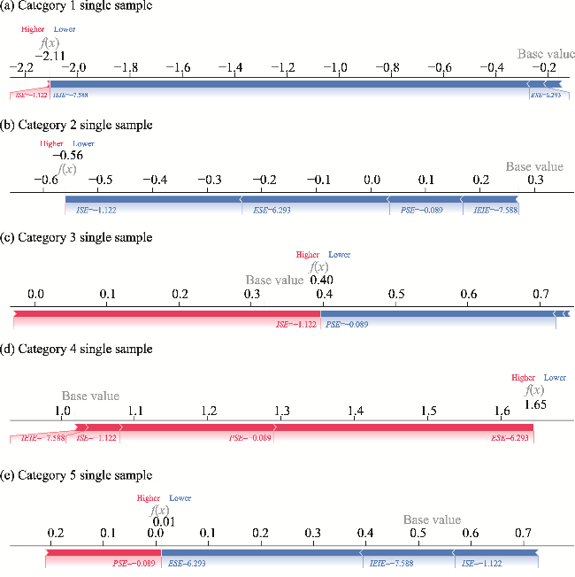
Figure 5 SHAP value single sample force plots by category |
Table 4 SHAP values of IEIE for the strong decoupling state (category five) from 2007 to 2021 |
| Year | Hohhot | Baotou | Hulunbeir | Hinggan | Tongliao | Chifeng | Xilin Gol | Ulanqab | Erdos | Bayannur | Wuhai | Alxa |
|---|---|---|---|---|---|---|---|---|---|---|---|---|
| 2007 | -0.176 | -0.096 | -0.206 | 0.039 | 0.086 | 0.085 | -0.028 | 0.065 | 0.030 | -0.014 | 0.068 | 0.040 |
| 2008 | -0.077 | -0.218 | -0.206 | 0.225 | 0.085 | -0.195 | 0.087 | 0.165 | -0.248 | 0.052 | 0.068 | -0.028 |
| 2009 | 0.059 | 0.060 | -0.236 | 0.133 | 0.085 | 0.083 | 0.068 | 0.065 | 0.030 | 0.078 | 0.087 | 0.038 |
| 2010 | 0.152 | 0.159 | -0.208 | 0.133 | 0.010 | 0.072 | -0.009 | 0.174 | 0.131 | -0.042 | -0.056 | 1.370 |
| 2011 | -0.077 | 0.089 | -0.196 | -0.014 | 0.085 | 0.083 | 0.184 | 0.072 | -0.206 | 0.052 | 0.075 | -0.024 |
| 2012 | 0.102 | 0.362 | 0.090 | -0.020 | 0.085 | 0.086 | 0.088 | 0.052 | -0.191 | 0.225 | 0.362 | 0.146 |
| 2013 | 0.060 | 0.362 | 0.165 | 0.133 | 0.334 | 0.254 | 0.254 | 0.133 | 0.102 | 0.133 | 0.172 | 0.159 |
| 2014 | -1.404 | 0.126 | 0.523 | 0.169 | 0.241 | 0.706 | 0.241 | 0.839 | 0.332 | 0.241 | 0.172 | 0.332 |
| 2015 | 0.907 | 1.266 | 1.477 | 1.356 | 1.356 | 1.276 | 0.151 | 1.356 | 0.913 | 1.235 | 0.157 | 1.370 |
| 2016 | -1.542 | 0.156 | 0.186 | 1.235 | 0.169 | 0.133 | 0.241 | 0.156 | 0.297 | 0.169 | 0.241 | 0.839 |
| 2017 | 0.362 | 0.387 | 0.359 | 0.133 | 0.334 | 0.359 | 0.403 | 0.334 | 0.214 | 0.334 | 0.334 | 0.359 |
| 2018 | -1.465 | -1.494 | -1.325 | -1.335 | -1.419 | -1.402 | -1.432 | -1.402 | -1.480 | -1.335 | -1.389 | -1.411 |
| 2019 | 0.210 | 0.164 | -1.401 | -1.427 | 0.241 | -1.370 | 0.527 | -1.303 | 0.625 | 0.169 | -1.366 | 0.034 |
| 2020 | -1.483 | -1.347 | -1.347 | -1.156 | -1.196 | -1.347 | -1.346 | -1.217 | -1.458 | -1.196 | 0.526 | -0.188 |
| 2021 | -0.017 | -0.233 | -0.006 | 0.225 | -0.116 | -0.115 | -0.233 | -0.228 | -0.219 | -0.115 | 0.042 | 0.094 |
| [1] |
|
| [2] |
|
| [3] |
|
| [4] |
|
| [5] |
|
| [6] |
|
| [7] |
|
| [8] |
|
| [9] |
|
| [10] |
|
| [11] |
|
| [12] |
|
| [13] |
|
| [14] |
|
| [15] |
|
| [16] |
|
| [17] |
|
| [18] |
|
| [19] |
|
| [20] |
|
| [21] |
|
| [22] |
|
| [23] |
|
| [24] |
|
| [25] |
|
| [26] |
|
| [27] |
|
| [28] |
|
| [29] |
|
| [30] |
|
| [31] |
|
| [32] |
|
| [33] |
|
| [34] |
|
| [35] |
|
| [36] |
|
| [37] |
|
| [38] |
|
| [39] |
|
| [40] |
|
| [41] |
|
| [42] |
|
| [43] |
|
| [44] |
|
| [45] |
|
| [46] |
|
| [47] |
|
| [48] |
|
| [49] |
|
/
| 〈 |
|
〉 |