Ecosystems and Ecosystem Services

Identification of Grassland Vegetation Coverage and Height Based on Vegetation Index and HSV Space

  • YANG Wenbo , 1 ,
  • GUAN Peng 3, + ,
  • SHI Honglei 2 ,
  • ZHANG Wei 3 ,
  • LEI Fuqiang , 3, *
Expand
  • 1. School of Mechanical Engineering, Hangzhou Dianzi University, Hangzhou 310018, China
  • 2. School of Technology, Beijing Forestry University, Beijing 100083, China
  • 3. School of Computer Science, Hangzhou Dianzi University, Hangzhou 310018, China
*LEI Fuqiang, E-mail:

+The author and the first author contributed equally to this work.

YANG Wenbo, E-mail:

Received date: 2024-10-23

  Accepted date: 2025-01-20

  Online published: 2025-08-05

Supported by

The Special Scientific Research Project Funds of China Electronics(631010703)

Abstract

In response to the demand for grassland vegetation monitoring, this study proposes a method based on the vegetation index and an automatic identification method of grassland vegetation coverage and height in the HSV color space. Hikvision smart ball machines and smartphones were used as fixed and mobile monitoring tools to conduct the experiments at the Sanqingyuan Nursery, Beijing Forestry University. Aiming at the time-series images from April to September 2021, five visible light vegetation indices, EXG, EXGR, NGRDI, GLI, and RGBVI, were comparatively analyzed in terms of vegetation coverage recognition. The experimental results show that the EXG index combined with the OTSU automatic threshold method has the best performance in extracting vegetation coverage, with an accuracy of 90% and an absolute error controlled within 3%; therefore, it was selected as the optimal algorithm. Second, this study converts the RGB color space into the HSV color space, realizes the accurate extraction of red color rings, and calculates the grass layer height accordingly. The experimental results show that the average error of this method is 2.3 cm, the maximum error is 6 cm, and the relative error is generally lower than 30%, indicating high reliability and accuracy. The results of this study provide an efficient and accurate automatic identification method for grassland vegetation monitoring and are expected to be widely used in grassland ecological protection and management.

Cite this article

YANG Wenbo , GUAN Peng , SHI Honglei , ZHANG Wei , LEI Fuqiang . Identification of Grassland Vegetation Coverage and Height Based on Vegetation Index and HSV Space[J]. Journal of Resources and Ecology, 2025 , 16(4) : 933 -945 . DOI: 10.5814/j.issn.1674-764x.2025.04.002

1 Introduction

With the rapid development of space technology, grassland monitoring has integrated remote sensing and other technical means, and even in remote areas that are difficult for humans to reach, large-scale grassland monitoring can be realized (Chen, 2008; Zhao et al., 2020). However, grassland monitoring cannot completely rely on remote sensing technology. Although the monitoring range is large, it has many disadvantages, such as low spatial resolution, ease of being affected by clouds, and large financial investment.
The methods for obtaining vegetation coverage in field measurements mainly include visual estimation, acupuncture, and the grid method. The objective estimation method is highly subjective and its maximum absolute error is as high as 40% (Coy et al., 2016). The acupuncture method uses the principle of probability, and the measurement results are more accurate; however, the efficiency is low, time-consuming, and labor-intensive. The grid method also uses the principle of probability and statistics to obtain the vegetation coverage, and the measurement accuracy varies with the total number of grids (Yang et al., 2021). The acupuncture method and grid method are limited by cumbersome operation, so they are not suitable for large spatial measurements, but they are still used in actual field investigations at present.
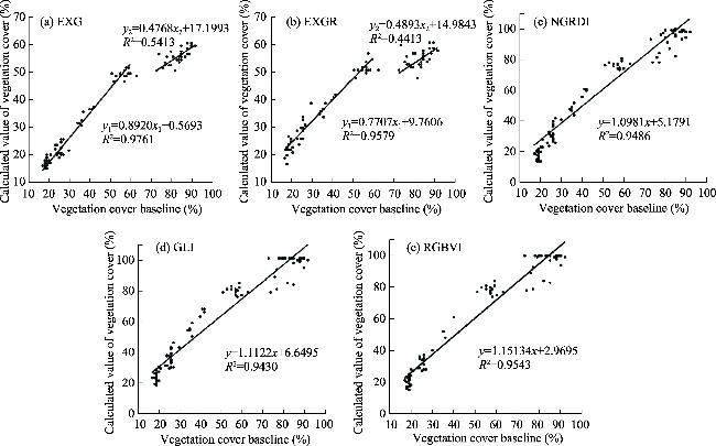
Vegetation cover recognition has mostly been studied with near-surface remote sensing images, using UAV or digital camera equipment to obtain high-resolution images, and then constructing vegetation indices in the visible band to extract the vegetation cover. Most researchers selected a variety of commonly used vegetation indices to compare the extraction effect; for example, the study of grassland in the school district selected four vegetation indices, and it was found that the cover extraction accuracy of the Vegetative Index (VEG) and EXG exceeded 93% (Fu et al., 2021). In karst and rocky desertification areas, the accuracy of the Excess Green Minus Excess Red Index (EXGR) reached 99.174% (Yin et al., 2020). Researchers have also proposed new vegetation indices, such as the New Green Red Vegetation Index (NGRVI), which was developed based on the construction principle of the Green Red Vegetation Index (GRVI) and Modified Green Red Vegetation Index (MGRVI), achieving an extraction accuracy of over 90% (Zhang et al., 2019). Additionally, the Excess Green-Red-Blue Difference Index (EGRBDI) was constructed by drawing on the Red Green Blue Vegetation Index (RGBVI), and its overall accuracy, applicability, and stability outperformed 18 other vegetation indices (Gao et al., 2020). The Difference Enhanced Vegetation Index (DEVI) was proposed with a supervised classification method based on Support Vector Machine (SVM) as the baseline for accuracy evaluation, showing significantly better extraction accuracy compared to eight other vegetation indices (Zhou et al., 2021). Furthermore, a novel approach was introduced by discarding traditional index construction forms and proposing a method to find the best index through function optimization, resulting in the DeepIndices model within a deep learning framework. This model is unaffected by external factors and monitoring shapes, offering better segmentation effects and stability (Vayssade et al., 2021). In addition to the vegetation index method, the Red, Green, Blue (RGB) decision tree method (Zhang et al., 
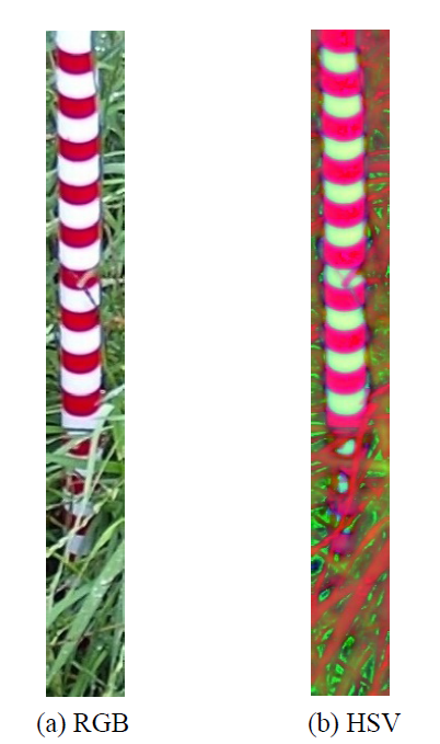
2013), the Hue, Saturation, Value (HSV) discriminant method (Chen et al., 2014), and the Lab color space a-component method (Xu et al., 2018) are commonly used, all of which have good extraction accuracy and can be quickly determined. All of the above belong to the image-oriented method, which is suitable for scenes with high image resolution and has the advantages of rapid determination, cost-effectiveness, efficiency, and accuracy compared with satellite remote sensing. However, this method separates image acquisition from cover extraction and requires centralized processing after acquiring images with a low degree of automation.
With the development of handheld mobile devices, the shooting ability of smartphones, tablets and other mobile devices has been greatly improved, and their resolution reaches ten million levels, which meets the shooting requirements of cover images, and they are beginning to be researched and applied in grassland field surveys. For example, to address the demand for real-time vegetation cover estimation in field surveys, a vegetation cover estimation application was developed based on the Android platform (Ding et al., 2017). Additionally, a collaborative acquisition system for mobile terminals was designed to facilitate data sharing during team-based vegetation cover collection (Dong, 2016). This approach resolves the issue of separating image acquisition from cover extraction and represents a potentially significant research direction.
Second, the height of the grass layer is usually obtained using the sampling method in a field survey. Along the two diagonal lines of the sample, 10 points were evenly selected to measure plant height, and the average value was taken as the height of the grass layer in this sample. Numerical values are often determined manually or after mowing; the former is simple but time-consuming, and the latter causes a certain degree of damage to the grass layer. To enable the rapid determination of grass yield, a grass measuring stick was developed, featuring a cylindrical design with a black-and-white banded scale and hay yield values. Experimental results demonstrated that this tool significantly reduces manpower and time compared to traditional sampling methods, while also providing a more user-friendly approach for grassland monitoring workers (Li et al., 2016). However, this method fails to detach from the subjectivity of the measurement and realizes an automatic measurement.
High-precision physical devices assist in the measurement of plant heights, allowing for precise measurements. For example, the application of ground-based LiDAR transforms the three-dimensional coordinates of plants into a three-dimensional object model, and the measurement accuracy can reach the centimeter level at the sample scale. Hao et al. combined light detection and ranging (LiDAR) with a UAV and proposed an Air-LiDAR grass canopy height estimation model, whose fitting results and coefficient of determination satisfied the test requirements and had good estimation accuracy (Hao et al., 2021). A point cloud processingff method based on laser altimetry was proposed, and the estimated canopy height showed consistency with LiDAR results (Wang et al., 2020). Although these methods can obtain more accurate results, they are too expensive and have limitations in field applications. However, they can only be used to obtain data during field surveys, and it is difficult to realize long-term continuous measurements.
With the development and application of image processing technology in various fields, the use of digital images to monitor plant height has become possible and is an important direction of research in this field. A digital camera mounted on a drone was used to photograph mossy landforms, resulting in the construction of a surface model with a resolution of 2 cm (Lucieer et al., 2014). Similarly, RGB images captured by a drone were utilized to construct a multi-temporal digital surface model with a resolution of less than 1 cm, effectively reflecting spatial and temporal changes in grass height (Bareth et al., 2019). Although this type of research reduces the measurement cost, the UAV platform is not well suited for continuous monitoring. A four-point identification and automatic calibration method was proposed for the automatic extraction of crop plant height using video cameras and digital image processing techniques, achieving remote automatic measurement of a single plant with an error of only 1.98% (Yan, 2016). Moreover, the EXG index was employed to segment corn images and extract corn feature images. The Zhang calibration method was used for camera calibration to achieve distortion correction, and a projected geometric model was constructed between the pixel points of the corn image and the camera imaging. This enabled the calculation of the actual height of corn plants in farmland backgrounds, leading to the design and construction of a corn plant height measurement system that significantly improved measurement accuracy and efficiency (Xing, 2020).
This study is aimed at the urgent need for grassland ground monitoring work, adopting two ways of fixed monitoring and mobile monitoring, researching and realizing the automatic recognition of grassland vegetation information based on digital images, the main recognition content including vegetation cover and grass layer height, realizing automated operation from the grassland vegetation image collection, to the acquisition of grassland vegetation information, and then to the grassland vegetation information into the database and release, and providing a new software platform for grassland monitoring and field investigation work to reduce the burden of annual dynamic monitoring to provide data results, and provide ideas for the construction of forest and grass sensing networks. It can reduce the burden of grassland monitoring field surveys, provide data results for annual dynamic monitoring of grassland, provide ideas for the construction of forest and grassland sensing networks, and provide a new software platform for grassland monitoring and informatization management.

2 Materials and methods

2.1 Overview of the study area

The experimental sample site was selected from the Sanqingyuan Nursery (40°00′28.22″N, 116°20′18.91″E) of the Beijing Forestry University. The site belongs to the warm temperate semi-humid and semi-arid continental monsoon climate zone with four distinct seasons. Spring is windy and arid, summer is hot and rainy, fall is windy and light, and winter is cold with little rain or snow. Precipitation due to the monsoon climate and annual seasonal changes are mostly concentrated in summer. The average annual number of days of precipitation was 66.8 days, the number of days of snowfall was 9-10 days, and the number of days of snow was approximately 11. The average number of sunshine hours was 2444.9 hours, and the percentage of sunshine was 60%. The average annual evaporation was 1900.4 mm. The main months of evaporation during the year were from April to June, with an average cumulative evaporation of 814.9 mm, and the average monthly evaporation was above 200 mm, accounting for 43% of the year.

2.2 Study objects

Most of the vegetation species in the sample plots were ryegrass, which is an excellent pasture grass commonly introduced and cultivated, preferring a cool and humid climate with a fast growth rate but poor growth above 35 ℃, and tillering will stop or die halfway if the temperature is too high.

2.3 Experimental fixed monitoring equipment

In this experiment, an intelligent dome camera (model: DS-2DE6C423IW-D/GLT) of the Hikvision E series was used as near-surface remote sensing equipment to photograph the growth of ryegrass. The near-surface remote sensing equipment was utilized to collect time-series images, and it was equipped with a maximum resolution of 2560×1440 pixels, 360° horizontal rotation, vertical direction of -15°-90° (automatic flip), normal operation under ambient temperature (-30 ℃-65 ℃), support for 30x optical zoom, 16x digital zoom, 3D digital noise reduction, glare suppression, and other functions. Since the fixed monitoring station was established in the nursery area, clean solar energy was used as the source of electricity, and the solar-powered equipment was selected, model HG240-24-120. The image samples selected for this study were the time-series of phenological images from April to September 2021, and one climatic image was captured every day at 10:00 and 16:00, and the resolution of the original image was 2560×1440 pixels, occupying a space between 1 MB and 1.5 MB. After image screening, blurred images that were not successfully focused and images that were obscured by masks were excluded, the continuity of the images was checked, and the vacant photos were interpolated by replacing the vegetation images with those of the closest time period. A total of 328 phenological images were collected on 164 days, and sample images were acquired, as shown in Figure 1.
Figure 1 Example of a phenological image taken by a fixed monitoring station

2.4 Experimental mobile monitoring equipment

The grassland vegetation information mobile monitoring system is primarily designed for field survey applications. Its core components include smartphones, specialized applications installed on these smartphones, and cloud servers, with the latter mainly serving as a database interface. Additionally, the system requires a grassland field survey sample frame and a handheld smartphone bracket to facilitate fieldwork. Modern smartphones with standard configura-tions, such as camera functionality, GPS positioning, and internet connectivity, are fully capable of supporting this system. The handheld smartphone bracket aids in capturing imagery by ensuring the smartphone is extended and parallel to the ground, enabling high-quality photographs of grassland vegetation. A physical representation of this setup is provided in Figure 2.
Figure 2 Hand-held mobile phone bracket

2.5 Vegetation index

The recognition of grassland vegetation cover based on RGB images fundamentally entails extracting all the image elements that signify the vegetated portion within the image. This is achieved by leveraging the image characteristics of both the vegetated and non-vegetated areas, segmenting the image and then binarizing it, ultimately leading to the successful identification of vegetation cover. The commonly employed image features include color features, texture features, shape features, and spatial relationship features. Among these, color features are element-based and typically associated with the objects or scenes present in the image. They exhibit insensitivity to alterations in the size, orientation, and viewing angle of the image. Moreover, in comparison to other features, they possess the advantages of requiring less computational effort and demonstrating high efficiency. Given the application context of the algorithm, the digital images captured and stored via near-ground remote sensing and smartphones are in the RGB color space. Consequently, this particular color space is opted for in the extraction of vegetation cover.
Visible vegetation indices, widely used in vegetation cover research, include the Excess Green Index (EXG), the Excess Green Minus Excess Red Index (EXGR), VEG, the Green Leaf Index (GLI), and the Combined Index (COM), among others. These indices are typically derived from combinations of red, green, and blue channel bands in an image. In this study, several commonly employed indices with varying construction principles—EXG, EXGR, the Normalized Green-Red Difference Index (NGRDI), GLI, and the Red-Green-Blue Vegetation Index (RGBVI)—are selected for experimental analysis. The detailed construction formulas for these indices are provided below.
① The Excess Green Index (EXG): Among the visible vegetation indices. Originally proposed by Woebbeeke et al. in 1995, it has gained significant attention and has been extensively studied and utilized by researchers worldwide. Its popularity stems from its effective application in the automatic separation of vegetation and soil (Woebbeeke et al., 1995). The formula for calculating EXG is as follows:
EXG=2GRB
where G, R, B denote the separate channels of the RGB image, representing the brightness values (Digital Numbers, DN values) of the green, red, and blue light bands for each pixel. These values range from 0 to 255.
② The Excess Green Minus Excess Red Index (EXGR): EXGR was introduced by Meyer et al. (2008). It refines vegetation analysis by subtracting the Excess Green Index (EXG) from the Excess Red Index (EXR), offering improved performance in separating vegetation from soil (Meyer et al., 2008). The formula for calculating EXGR is:
EXGR=3G2.4RB
③ The Normalized Green-Red Difference Index (NGRDI): NGRDI focuses on the green and red light bands. It calculates the difference between these bands and normalizes the result to a range of -1 to 1. Developed by Hunt et al. in 2005, this index identifies vegetated areas with positive values, while negative values indicate soil or non-vegetated areas (Hunt et al., 2005). Its calculation method is as follows:
NGRDI=GRG+R
④ The Green Leaf Index (GLI): GLI was proposed by Louhaichi et al. in 2001. It measures the difference between the green light band and the combined red and blue light bands, normalized to a range of -1 to 1. Like the NGRDI, positive GLI values signify vegetated areas, while negative values indicate non-vegetated areas (Louhaichi et al., 2001). The formula is as follows:
GLI=2GRB2G+R+B
⑤ The Red-Green-Blue Vegetation Index (RGBVI): RGBVI effectively identifies vegetation by combining the reflectance of red, green, and blue bands and squaring the green band’s DN value to highlight vegetation’s strong reflectance in green light (Guerrero et al., 2012). While accurate, its performance decreases in areas with sparse vegetation. The RGBVI calculation method is:
RGBVI=G2R×BG2+R×B

2.6 Threshold segmentation and maximum interclass variance methods

After enhancing the green vegetated regions in the image using the five vegetation indices discussed above, the color features of the image become more distinct. This allows for image segmentation to effectively separate vegetated and non-vegetated areas. Image segmentation involves dividing an image into specific regions with unique properties to isolate the target of interest. According to Huang Peng et al. (2020), segmentation methods can be broadly categorized based on theories such as thresholding, regions, and edges. Among these, threshold segmentation is the simplest and most efficient method. Its principle involves classifying the grayscale histogram of an image by applying various thresholds, where elements within the same grayscale range are grouped into a single class due to their similarity.
The key to threshold segmentation lies in selecting an appropriate threshold value. In this study, the automatic recognition of grassland vegetation cover is conducted. Since the vegetation images are captured in a natural environment, they are influenced by factors such as natural light, shading, and shadows, which cause variations in the Digital Number (DN) values corresponding to brightness. As a result, a fixed threshold value cannot meet the system’s requirements. Therefore, the Maximum Inter-Class Variance method, also known as Otsu’s method, is employed to determine an adaptive threshold value, enabling automatic segmentation.
The Maximum Inter-Class Variance method is widely used in digital image processing and is considered one of the most effective algorithms for selecting threshold values in image segmentation. It is simple to compute and remains unaffected by variations in brightness and contrast. The method calculates the inter-class variance for all gray levels in the image, and the gray level with the largest inter-class variance is identified as the optimal threshold. Once the optimal threshold value is determined, the image can be binarized: pixel values corresponding to the vegetation, with gray values greater than the threshold, are set to 1 (white), while pixel values corresponding to non-vegetation, with gray values smaller than the threshold, are set to 0 (black).
After completing the image segmentation, vegetation cover recognition involves calculating the percentage of pixels corresponding to the vegetated area relative to the total number of pixels in the image. This can be computed using the following formula:
$\text { Vegetation cover }=\frac{N^{\prime}}{N} \times 100 \%$
where Nʹ and N represent the number of pixels in the vegetation area and the total number of pixels in the image, respectively.

2.7 Vegetation image preprocessing

The sample box in the original image appears as a bright white square, which contrasts clearly with the surrounding vegetation and soil. After overlaying the R-component map with the B-component map, the brightness difference between the sample box area and the surrounding regions becomes even more pronounced, as shown in Figure 3.
Figure 3 Overlay of R and B component image
Automatic threshold segmentation is applied to the R+B component overlay map, resulting in a binary image that only includes the sample box region. Next, the Hough Transform is used to detect four straight lines, which form the contour of the sample box, as shown in Figure 4a. In Figure 4b, rectangular contour detection is performed, and the detected rectangle is filled to create a mask. The mask is then applied to the original image using logical operations, as shown in Figure 4c, to obtain the Region of Interest (ROI), thus completing the image preprocessing for the mobile monitoring system.
Figure 4 Extraction process of Region of Interest (ROI)

3 Results

3.1 Research area selection

Before recognizing grassland vegetation information, it is essential to preprocess the vegetation image, extract the ROI, and highlight the key areas to reduce processing time and improve recognition accuracy.
The images captured by the fixed monitoring system and the mobile monitoring system differ slightly in size and preprocessing steps. In the fixed monitoring system, the original vegetation image, captured by near-ground remote sensing, has a resolution of 2560×1440 pixels. The content is captured at a fixed angle using the smart dome, so the ROI is predetermined, and only a fixed area needs to be cropped during preprocessing. In contrast, for mobile monitoring, due to the variability in sample locations, the field survey sample box is typically used to demarcate the sample area and capture vegetation images, as shown in Figure 5.
Figure 5 Original images taken by the mobile monitoring system
The size of the original vegetation image captured by the mobile monitoring system is related to the shooting capabil-ity of the smartphone equipped with the application. In the vegetation image, the area within the sample box is the ROI, so when the image preprocessing extracts the ROI, it is necessary to carry out the sample box identification.

3.2 Methods of vegetation cover baseline value

The true value of vegetation cover is difficult to obtain, and in practical grassland surveys, methods based on statistical principles, such as the needle method and grid method, are commonly used to estimate the “real value.” With the widespread use of photographic techniques, vegetation images are now captured during external surveys, while vegetation cover identification is often performed internally. This process typically involves methods such as manual outlining (e.g., using Photoshop), software simulations of the pin- prick method, the image grid method, and supervised classification techniques (Zhang et al., 2010; Yang et al., 2021).
Due to the predominantly long and narrow shape of vegetation leaves in the experimental area, implementing the manual outlining method proves challenging. Therefore, this experiment adopts the grid method. The ROI image is divided into a 20×20 grid to calculate the baseline value of vegetation cover, as shown in Figure 6. Each grid is evaluated, and grids where vegetation occupies at least half of the area are counted. The baseline vegetation cover value is then determined as the percentage of grids containing vegetation relative to the total number of grids.
Figure 6 20×20 grid density schematic

3.3 Vegetation cover identification experiment

The fixed monitoring and mobile monitoring systems are designed to use the same algorithm, with this experiment focusing solely on the vegetation cover recognition method. For the study, 100 vegetation images were selected, with cover values ranging from 10% to 100%. Each image was preprocessed to a size of 1000×1000 pixels, corresponding to an actual area of 50 cm×50 cm within the sample square.
Vegetation indices were extracted from the vegetation images using Equations 1-5 and subsequently mapped to grayscale to generate single-channel grayscale images, as illustrated in Figure 7.
Figure 7 Gray scale images of vegetation indexes
As shown in Figure 8, the grayscale images reconstructed using the five vegetation indices effectively distinguish between vegetated and non-vegetated areas. Among these, the grayscale maps derived from EXG and EXGR indices exhibit significant contrast, with the vegetated areas appearing at a higher gray level compared to non-vegetated areas. This strong contrast is advantageous for vegetation image segmentation. In contrast, the grayscale maps of NGRDI, GLI, and RGBVI indices show minimal differences in gray levels, making them less suitable for automatic threshold segmentation.
Figure 8 Binary images of vegetation indexes
To address this, the EXG and EXGR vegetation indices were binarized using the OTSU method, while the NGRDI, GLI, and RGBVI vegetation indices were binarized using a 0-threshold method. The resulting binary images are presented in Figure 8.
Figure 8 shows that all indices effectively separate vegetation from the background. However, the vegetation areas identified using the 0-threshold method are slightly larger than those identified using the OTSU method. This discrepancy arises because the 0-threshold method is less effective at recognizing the edges of green vegetation and tends to classify shaded regions in dense vegetation areas as part of the vegetation. As a result, the calculated values tend to be overestimated.
After completing threshold segmentation, each pixel in the binary image is traversed to count the total number of pixels in the vegetation region. The vegetation cover value is then calculated using Equation (6), providing the final vegetation cover recognition results.

3.4 Grass layer height recognition

The mobile monitoring system does not involve grass layer height recognition, which can be directly measured on-site; therefore, the study only focuses on extracting grass layer height using digital images in a fixed monitoring system. To reduce the construction cost of the fixed monitoring station, the height of the grass layer was measured using a self-made height measuring pole. The body of the height measuring pole was equipped with a red and white 1 cm wide color ring, which was inserted into the grass layer to shoot the image of the pole, extract the number of red rings in the image that were not completely blocked by the grass layer, and then convert the height of the grass layer to convert the grass layer height extraction problem into a number of red color rings extraction problem, so as to realize the automatic recognition of the height of the grass layer.

3.4.1 RGB color space and HSV color space

To facilitate the identification of the scale color ring of the height measuring pole, the image must contain only the vegetation part and the height measuring pole. To avoid the influence of other complex environments, the scale color ring of the height measuring pole was set to red and the green vegetation to form a clear distinction. The height measuring pole image captured by the smart dome is an RGB image, which represents the color through a linear combination of red, green, and blue components. Any color is related to the three components, which makes it difficult to digitally adjust the details, and the extraction of the red ring is more difficult to achieve. By contrast, the HSV color space is more advantageous for extracting a single-color feature, which consists of three parameters: hue (H), saturation (S), and lightness (V). It can intuitively express the hue, vibrancy, and lightness of the color, making it easier to track a certain color than in the RGB color space, and it is the best choice for extracting the red color ring.
To ensure the convenient identification of the scale color ring on the height measuring pole, it is necessary for the image to solely comprise the vegetation portion and the height measuring pole, thereby eliminating interference from other complex surroundings. The scale color ring of the height measuring pole was designated as red to create a distinct contrast with green vegetation. The image of the height measuring pole captured by the smart dome is in the RGB format, where the color is represented by a linear combination of red, green, and blue color components. Because any color is related to these three components, it is challenging to digitally adjust the details precisely, and extracting the red ring is particularly arduous. In comparison, the HSV color space has a greater advantage for extracting a single color feature. By comparing H, S, V, we can vividly express the hue, intensity, and brightness of the color. Moreover, it is more convenient to track a specific color within the HSV color space than within the RGB color space, making it the optimal option for extracting the red ring.
The conversion from RGB color space to HSV space can follow the following formulas:
Max=max(R,G,B)Min=min(R,G,B)
H=0°, Max=Min                                 GBMaxMin×60, R =Max                BR MaxMin×60+120, G=Max RG MaxMin×60+240, B =Max
S=MaxMinMax
V=Max
In the above Equations, H, S, and V represent the hue value, saturation value, and brightness value of each pixel in the image, respectively.
The R in the HSV color space corresponds to the value ranges of [0,43,46]-[10,255,255] and [156,43,46]-[180,255,255]. After converting the height-measuring pole image into an HSV image, all red ring regions can be extracted based on the above ranges. After converting the altimetry riser image to the HSV image, all the red-ring regions can be extracted according to the above ranges.

3.4.2 Contour extraction and color ring counting

After the red part is extracted under the HSV color space, the image consists of only the red and non-red parts, which are further distinguished using a binarized image. The color ring that is not obscured by the grass layer is presented as a white-connected domain after binarization, and the height of the grass layer can be deduced by counting the number of complete color rings. However, the machine cannot solve the seemingly simple manual counting problem, and the use of image processing methods to count the number of complete color rings also needs to follow the method below.
First, we need to determine the number of white-connected domains in the binary image. Boundary tracking is a basic image processing technique that extracts boundary contours as a series of coordinate points or chain codes (Suzuki and Abe, 1985). The encircling relationship between the outer and hole boundaries can be extracted using image topology, transforming a binary image into a boundary description. In this method, there are strictly no holes in the connected domain extracted from the image; therefore, it is sufficient to extract only the outer layer contour. There exists a contour extraction function findContours() in OpenCV, which helps to detect the outer contours of all connected domains in a binary image and obtain all the coordinate values of each contour and the total number of contours, that is, the number of white connected domains. Then, traversing each contour, calculating the area occupied by each connected domain, setting the minimum area of the complete color ring as the comparison value, comparing it with the area of connected domains, recording the connected domains that are larger than the comparison value, and then counting the number of connected domains that represent the complete color ring.
Setting the height of the height measuring pole in the ground part as Hground, the vegetation growth will cover part of the height measuring pole; the number of color rings in the uncovered part is set as N, the red ring of the height measuring pole is 1 cm wide, and the interval between the two color rings is 1 cm, so the height of the grass layer Hg, can be deduced by the following formula:
Hg=Hground-2N

3.5 Grass layer height recognition experiment

This experiment explored an automatic grass layer height recognition algorithm for a fixed monitoring system. Thirty altimetry riser images were selected for the experiment, and the actual height of the grass layer in the images ranged from 1 to 40 cm. The original image resolution of the sample images was 2560×1440 pixels, and the occupied space was between 1 MB and 1.5 MB.
First, the original altimetry riser image was preprocessed to extract the ROI. Because the original image contains too many environmental elements, to ensure the efficiency and accuracy of grass layer height recognition, the original image was cropped to a fixed area, and the ROI obtained contained only the complete height measuring pole and some green vegetation, which is convenient for image processing. After extracting the ROI, the image size was 75×650 pixels so that the processing target focused on the altimeter pole, which reduced the scale of the recognition algorithm and shortened the recognition speed.
After obtaining the ROI, in accordance with Equations (7)-(10), the ROI is converted to color space, from RGB space to HSV space, Figure 9 shows the image comparison after the ROI color space conversion. Figure 9a RGB image, after ROI extraction to remove the complex background effects, the naked eye can distinguish the obvious red color ring, but it is difficult to completely extract the red color by image processing methods. Figure 9b HSV image after color space conversion, where the white part corresponds to the red ring in the RGB image, and there is an obvious difference with the non-color ring region. This figure only shows a comparison of the effect before and after the conversion space, that is, the actual program run, according to the coordinates of the converted HSV image to determine the red ring in the region.
Figure 9 Comparison of RGB image and HSV image
According to the corresponding range of the red color in the HSV model, the inRange() function is used to create two mask masks based on the HSV image, respectively, and the two masks are then summed to form a single-channel red color-ring bivariate map, as shown in Figure 10a.
Figure 10 Binary segmentation and contour extraction
The white contiguous domains in the binary map are color rings that the vegetation fails to obscure, including complete and incomplete color rings. The contours of each connected domain were extracted using the findContours() contour-discovery function. Each contour was traversed and the area of each connected domain was calculated separately. After calibration, the minimum complete color ring area was determined and compared to the area of each contiguous domain. The contiguous domains whose areas were smaller than the specified value were removed, and the number of complete color rings was counted. The drawContours() function was used to draw the blue contours of the complete color ring in the ROI image to verify the effect, as shown in Figure 10b.
The number of complete color rings is obtained after image processing, and the value is brought into Equation 11 to derive the value of the grass layer height of this image, which is used as the final result of automatic identification of the grass layer height.

3.6 Vegetation cover recognition results and accuracy evaluation

After calculating the benchmark value for all sample images using the grid method, the scatterplot was plotted and linear regression was performed using the benchmark value as the horizontal axis and the calculated value of each vegetation index recognition as the vertical axis to compare the ability of several vegetation indices to extract the vegetation cover.
As shown in Figure 11, the scatter distribution of EXG and EXGR is divided into two parts; before the benchmark value is 70%, i.e., when the vegetation cover is below 70%, the difference between the calculated value and the benchmark value is not very large; however, after the benchmark value reaches 70%, the vegetation cover computed by EXG and EXGR indices is much smaller than the benchmark value. Therefore, in the linear regression of these two indices, the 70% vegetation cover benchmark value was used as the boundary, and the linear regression of these two components was carried out separately. This is not the case for NGRDI, GLI & RGBVI.
Figure 11 Linear regression of vegetation indexes
From the scatter distribution and correlation coefficient R2, the scatters of EXG and EXGR index automatic threshold segmentation methods are more densely distributed near the regression line, and the R2 is 0.9761 and 0.9579, respectively, which indicates that the extraction results have strong correlation with the baseline value; the correlation coefficients of the two are only 0.54 and 0.44 when the baseline value is greater than 70%, this is because when the vegetation cover is large Using the grid method will overestimate the size of the vegetation cover to some extent, and the automatic threshold segmentation method will underestimate it, so it causes this phenomenon, and this part is not taken into account when calculating the accuracy. While the R2 of the segmentation method of NGRDI, GLI and RGBVI index based on 0 threshold is around 0.95, the extraction results still have some correlation with the benchmark value, but the consistency is poorer compared to EXG and EXGR, and the scatter of the benchmark value at 40%-60% is concentrated above the regression line, and the segmentation result is large overall.
In terms of regression slope, the regression slopes of NGRDI, GLI, and RGBVI indices are all greater than 1, and their extracted vegetation cover values are overestimated to a certain extent compared with the baseline values, especially in the images with the baseline values of 40%-60%. While the regression slopes of EXG and EXGR indices are all less than 1, the results are low compared to the benchmark value, the reason is that both indices are segmented by OTSU automatic thresholding method, which is insensitive to slender vegetation as well as non-green vegetation, which can be interpreted when acquiring the benchmark value.
Linear regression can be more intuitive to see whether the trend of change between the calculated value and the benchmark value is consistent or not, and cannot show the accuracy of the calculated value, in order to objectively and quantitatively evaluate the effect of each type of vegetation index to identify the vegetation cover introduces the accuracy F evaluation standard, and its specific calculation formula is as follows:
F=1XiXX×100%
where Xi is the calculated value identified by the vegetation index method and X is the baseline value obtained by the grid method.
Table 1 for the comparison of the recognition accuracy of each vegetation index, the recognition accuracy of GLI, NGRDI and RGBVI indexes are not high, all below 80%, and the accuracy of EXG index is the largest, and the absolute error is about 3%, the calculation result is more stable, and the optimal extraction effect can be obtained.
Table 1 Identification results of each vegetation index
Vegetation index Mean absolute error Precision (%)
EXG 0.028 90
EXGR 0.016 86
NGRDI 0.099 75
GLI 0.121 71
RGBVI 0.098 77
Based on the experimental results, EXG index combined with OTSU method was finally selected as the grassland vegetation cover recognition algorithm. The accuracy of this method is within the acceptable range, and it can satisfy the demand for rapid, batch and automated extraction of grassland vegetation cover from server and cell phone at the same time.

3.7 Grass height recognition

Taking the grass height of the sample images recognized by the above experiments as the calculated value, the real value of the grass height is obtained by manual observation, the method is to manually count the total number of white and red color rings, and the grass height is deduced by the principle of Equation (12), which is used as the reference value for the evaluation of recognition accuracy. The results are shown in the Table 2.
Table 2 Results of grass layer height extraction
Image number Reference point (cm) Effective
number of rings
Measured value (cm) Absolute
error (cm)
Relative
error (%)
1 1 38 2 1 100.00
2 2 38 2 0 0.00
3 7 34 10 3 42.86
4 8 33 12 4 50.00
5 8 34 10 2 25.00
6 9 34 10 1 11.11
7 9 33 12 3 33.33
8 10 34 10 0 0.00
9 10 33 12 2 20.00
10 10 34 10 0 0.00
11 12 34 10 2 16.67
12 13 34 10 3 23.08
13 14 33 12 2 14.29
14 15 30 18 3 20.00
15 16 31 16 0 0.00
16 16 28 22 6 37.50
17 18 29 20 2 11.11
18 19 28 22 3 15.79
19 19 29 20 1 5.26
20 21 28 22 1 4.76
21 22 27 24 2 9.09
22 24 30 18 6 25.00
23 28 23 32 4 14.29
24 28 26 26 2 7.14
25 28 22 34 6 21.43
26 34 21 36 2 5.88
27 38 21 36 2 5.26
28 40 18 42 2 5.00
29 41 18 42 1 2.44
30 42 17 44 2 4.76
As can be seen from Table 2 with the help of image automatic identification of grass layer height compared with the results of manual observation, the maximum error value can be up to 6 cm, the average error is 2.3 cm, the relative error except for a few cases generally below 30%. This is because the index value of the measuring tool determines the accuracy of the measurement, the red color ring itself is 1 cm wide, the interval between the two is 1 cm, in the manual observation, the red and white ring can be read, while the image recognition can only read the red color ring, and the environment will have a certain impact on the image processing.
The reference value and the automatic recognition calculation value do linear regression, as shown in Figure 12, its regression slope is close to 1, and the R2 is 0.95, which proves that the calculation value has certain reliability and accuracy. Therefore, the system adopts this algorithm for automatic identification of grass layer height in practical application has feasibility.
Figure 12 Linear regression of grass height reference values on calculated values

4 Conclusions

This study details the methodology, experimental processes, and analysis of results related to identifying grassland vegetation cover and grass layer height. For vegetation cover identification, five visible light vegetation indices were assessed, and a 20×20 grid density was applied to establish baseline values. After performing linear regression and accuracy comparisons, the EXG index (with a 90% accuracy rate) and the OTSU automatic threshold method were selected as the most effective algorithms for extracting vegetation cover in both stationary and mobile monitoring systems. For grass layer height measurement, the color space was converted to HSV to simplify the extraction of the red color ring. The experiments demonstrated the practicality of a homemade height-measuring pole, achieving an average error of 2.3 cm and a maximum error of 6 cm—both within acceptable limits.
[1]
Bareth G, Lussem U, Menne J, et al. 2019. Potential of non-calibrated UAV-based RGB imagery for forage monitoring: Case study at the RENGEN long-term grassland experiment (RGE), Germany. The International Archives of Photogrammetry, Remote Sensing and Spatial Information Sciences, 42: 203-206.

[2]
Chen Q G. 2008. Current status and development of grassland monitoring in China. Pratacultural Science, (2): 29-38. (in Chinese)

[3]
Chen Z G, Batu N C, Xu Z Y, et al. 2014. Comparative study of grassland vegetation cover measurement methods based on digital camera. Acta Prataculturae Sinica, 23(6): 20-27. (in Chinese)

[4]
Coy A, Rankine D, Taylor M, et al. 2016. Increasing the accuracy and automation of fractional vegetation cover estimation from digital photographs. Remote Sensing, 8(7): 474. DOI: 10.3390/rs8070474.

[5]
Ding X, Qiu X F, Gao J Q, et al. 2017. Research on the estimation method of grassland vegetation cover based on cell phone photos. Zhejiang Journal of Agriculture, 29(6): 1017-1025. (in Chinese)

[6]
Dong Q. 2016. Design and realization of cooperative grassland information collection system based on mobile terminal. Diss., Beijing, China: China University of Mining and Technology. (in Chinese)

[7]
Fu S, Zhang Y H, Li J L, et al. 2021. Effects of different vegetation indices and drone altitude on the estimation accuracy of grassland cover. Pratacultural Science, 38(1): 11-19. (in Chinese)

[8]
Gao Y G, Lin Y H, Wen X L, et al. 2020. Recognition of vegetation information in visible light band based on UAV images. Transactions of the Chinese Society of Agricultural Engineering, 36(3): 178-189. (in Chinese)

[9]
Guerrero J M, Pajares G, Montalvo M, et al. 2012. Support vector machines for crop/weeds identification in maize fields. Expert Systems with Applications, 39(12): 11149-11155.

[10]
Hao X, Huang P P, Guo L B, et al. 2021. Research on airborne LiDAR grassland vegetation canopy height inversion method combined with topographic mapping data. Journal of Inner Mongolia Normal University (Natural Science Edition), 50(4): 299-307. (in Chinese)

[11]
Huang P, Zheng Q, Liang C. 2020. A review of image segmentation methods. Journal of Wuhan University (Natural Science Edition), 66(6): 519-531. (in Chinese)

[12]
Hunt E R, Cavigelli M, Daughtry C S, et al. 2005. Evaluation of digital photography from model aircraft for remote sensing of crop biomass and nitrogen status. Precision Agriculture, 6(4): 359-378.

[13]
Li W, Cao W M, Li X L, et al. 2016. Design and testing of a tool for rapid determination of grass yield in alpine grassland. Acta Agrestia Sinica, 24(4): 892-894. (in Chinese)

[14]
Louhaichi M, Borman M M, Johnson D E. 2001. Spatially located platform and aerial photography for documentation of grazing impacts on wheat. Geocarto International, 16(1): 65-70.

[15]
Lucieer A, Turner D, King D H, et al. 2014. Using an Unmanned Aerial Vehicle (UAV) to capture micro-topography of Antarctic moss beds. International Journal of Applied Earth Observation and Geoinformation, 27: 53-62.

[16]
Meyer G E, Neto J C. 2008. Verification of color vegetation indices for automated crop imaging applications. Computers and Electronics in Agriculture, 63(2): 282-293.

[17]
Suzuki S, Abe K. 1985. Topological structural analysis of digitized binary images by border following. Computer Vision Graphics & Image Processing, 30(1): 32-46.

[18]
Vayssade J A, Paoli J N, Gée C, et al. 2021. DeepIndices: Remote sensing indices based on approximation of functions through deep-learning: Application to uncalibrated vegetation images. Remote Sensing, 13(12): 2261. DOI: 10.3390/rs13122261.

[19]
Wang Y, Li S, Tian X, et al. 2020. Orientation-adaptive canopy height estimation of vegetation from satellite-based photon counting laser altimetry. Journal of Infrared and Millimeter Waves, 39(3): 363-371. (in Chinese)

[20]
Xing H R. 2020. Research on key technology of remote measurement system for corn plant height. Diss., Hefei, China: Anhui Agricultural University. (in Chinese)

[21]
Xu J Q, Qiu X F, D X, et al. 2018. Comparison of rapid extraction methods for grassland vegetation cover based on digital photographs. Jiangsu Journal of Agricultural Sciences, 34(2): 313-319. (in Chinese)

[22]
Yan J C. 2016. Remote automatic monitoring technology of crop canopy cover and plant height. Diss., Hangzhou, China: Zhejiang University of Technology. (in Chinese)

[23]
Yang Q, Pu H M, Zhao X C, et al. 2021. Comparison of field measurements of vegetation cover in three artificial grasslands. Journal of Applied and Environmental Biology, 27(1): 220-227. (in Chinese)

[24]
Yin L J, Zhou Z F, Li S H, et al. 2020. Study on vegetation information extraction and coverage in karst areas based on UAV visible light images. Acta Agrestia Sinica, 28(6): 1664-1672. (in Chinese)

[25]
Zhang Q P, Zhang S S, Chen L, et al. 2010. Application of WinCAM software to discriminate and analyze lawn cover. Pratacultural Science, 27(7): 13-17. (in Chinese)

[26]
Zhang C B, Li J L, Zhang Y, et al. 2013. A rapid method for quantitative determination of grass cover based on RGB model. Acta Prataculturae Sinica, 22(4): 220-226. (in Chinese)

[27]
Zhang X, Zhang F, Qi Y, et al. 2019. New research methods for vegetation information extraction based on visible light remote sensing images from an unmanned aerial vehicle (UAV). International Journal of Applied Earth Observation and Geoinformation, 78: 215-226.

[28]
Zhao L L, Zhang Y T, Zhang L, et al. 2020. Current situation, problems and countermeasures of grassland survey and monitoring in China. Forestry Construction, (6): 8-12. (in Chinese)

[29]
Zhou T, Hu Z Q, Han J Z, et al. 2021. Green vegetation extraction based on UAV visible light images. China Environmental Science, 41(5): 2380-2390. (in Chinese)

Outlines

/