Special Column: Ecotourism and Rural Revitalization

Spatial Structure of Tourist Attractions and Its Influencing Factors in China

  • WANG Zi , *
Expand
  • Faculty of Hospitality and Tourism Management, Macau University of Science and Technology, Macao 999078, China
*WANG Zi, E-mail:

Received date: 2024-09-01

  Accepted date: 2024-12-20

  Online published: 2025-08-05

Abstract

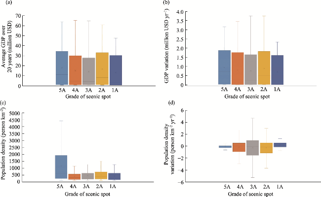
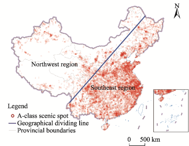
The complex types and regional differences in tourist attractions mean that the evaluation and quantification of spatial structures require inter- and trans-disciplinary methodologies. Previous studies on spatial structure have mostly focused on the law of tourist flow and the development trend of tourism, emphasising humanistic and economic methods. Currently, the main challenge of spatial structure research is the integration of natural, economic, and social factors and scientifically supporting tourism planning and management. From the perspective of geographical distance and geometric space, this study developed a quantitative method for the spatial structure of tourist attractions, which combines a grade classification index, spatial relationship function, and influence factor analysis and selects cases for implementation in a geographic information system, with the advantages of visualisation, timely data update, and convenient guidance for practice. It provided new insights for understanding the sustainable management of tourist attractions from the intersection of geography and tourism science. The research results indicate that China has the highest number of 4A and 3A level tourist attractions, accounting for 80.9% of the total. The nearest neighbor ratio of scenic areas is less than 1, showing a significant spatial distribution clustering pattern, with four major scenic area clusters located in eastern and southern China. The Natural environment determines the spatial layout of scenic areas, with 51.46% of scenic areas distributed in regions below 200 m in altitude, and 95.10% of scenic areas located in areas with a slope of less than 15 degrees. 1A and 2A level scenic areas are mainly distributed in cold and dry regions, while 5A, 4A, and 3A level scenic areas are relatively concentrated with similar climatic characteristics. 5A level scenic areas have higher GDP, population density, and growth rates. The spatial structure of scenic areas is closely related to population distribution and economic development; southeastern China accounts for more than 90% of the national population and GDP, and this region has over 60% of A-level and above scenic areas.

Cite this article

WANG Zi . Spatial Structure of Tourist Attractions and Its Influencing Factors in China[J]. Journal of Resources and Ecology, 2025 , 16(4) : 1079 -1088 . DOI: 10.5814/j.issn.1674-764x.2025.04.013

1 Introduction

An increasing number of countries emphasise the protection of the ecological environment, the coordination of economy, society, and culture, and the sustainable acquisition of economic benefits in tourism development (Budeanu et al., 2016). Assessing the quality, spatial distribution, and factors influencing regional tourist attractions forms the basis for scientific planning and effective management (Hu et al., 2024). Since 2003, China has formulated national standards pertaining to the classification, surveying, and evaluation of tourist attraction, with a revision undertaken in 2017. Existing studies have mainly focused on the classification of tourist attractions, the evaluation of scientific and humanistic values, environmental capacity, and service level (Scott et al., 2004; Zhan et al., 2015; Mangubhai et al., 2020; Arya et al., 2024).
According to the way of occurrence, tourist attractions are usually divided into two types: permanent and consumable. Resource attributes can be divided into natural and artificial tourism. Tourist motivation can be divided into four types of tourist attractions: Psychological, spiritual, fitness, and economic (Guo et al., 2000; Bafaluy et al., 2014). Spain’s national tourism census and classification system is highly recognized, and tourist attractions are divided into three primary types—natural landscape, architectural cultural landscape, and traditional customs—and seven secondary types and 44 tertiary types (Guo et al., 2000; Carrillo and Jorge, 2017; Alcalá-Ordóñez et al., 2023).
Owing to the complex types of tourist attractions and the diversification of tourists’ preferences, the quality evaluation and classification of tourist attractions face many challenges (Firdaus et al., 2018; Kim and Kang, 2022). The most prevalent methods construct evaluation indicators, assign weights according to the scores obtained by experts, and evaluate or grade the quality according to the scores obtained (Arya et al., 2024). The rationality of the index selection and the difficulty of quantifying some indices remain the primary issues. The monetary value evaluation of tourist attractions mainly includes two aspects: One expressed by shadow price and consumer surplus and the other by payment willingness-conditional value method (Machairas and Hovardas, 2005; Chang et al., 2021).
The spatial structure of tourist attractions is the basic parameter for describing and understanding tourism activities and is an important basis for coordinating environmental capacity and tourism scale (Könnyid et al., 2022; Wang et al., 2022). Some studies have focused on the scale and change of tourist behaviour or tourist flow and proposed a network spatial structure model composed of a mobility mode (convergence type, topology type), route, and crossover node (Balbi et al., 2013; Baum et al., 2017; Dong et al., 2023). The development of mathematical and geographic methods to describe various spatial structures has attracted considerable research attention (Novianti et al., 2020; Tsilimigkas and Rempis, 2021). Using spatial structure and dynamics to develop tourist behaviour, type, and geographical distribution models is important for explaining the evolution process of destination tourism (Balbi et al., 2013; Kim et al., 2020). The core-periphery model emphasises the dependence of periphery areas on core areas in tourism behaviour and is widely used in tourism planning (Barbero and Zofío, 2016). A point-axis relationship analysis can show the process of developing isolated tourist destinations into a certain spatial network structure (Aminu et al., 2013; Roman et al., 2020). When discussing tourism planning, Douglas (1995) divided space into three levels according to scale: national, regional, and local levels. From the perspective of supply and demand balance, some scholars have analyzed tourism supply space and demand space (Biagi and Pearce, 2010; Sarrión-Gavilán et al., 2015). Based on the sensitivity of tourists’ travel space to distance, studies have found that the longer the distance, the larger the scope and scale of tourists’ activities, and the shorter the distance, the higher the frequency of tourists’ visits to tourist objects (McKercher and Lau, 2008; Sano et al., 2024). Single sightseeing content can only attract close tourists, whereas excellent sightseeing content can attract numerous tourists (Richards, 2002; McKercher, 2017). In general, most existing studies on tourism spatial structure focus on the scale and change in tourist behaviour or tourism flow (Mazanec, 1983; Lin and Kuo, 2016; Bowen, 2022).
Previous studies on tourist attractions and their spatial structures have laid important methodological foundations and planning practices. From the perspective of geography, this study combined hierarchical analysis, average nearest neighbour and kernel density methods to determine the spatial structure of tourist attractions (SSTA), and integrated geographic information system technology, and utilized a comprehensive sample of A-level scenic spots to uncover their temporal-spatial characteristics and underlying mechanisms.

2 Material and methods

2.1 Framework for quantifying the spatial structure of tourist attractions

The proposed framework for the SSTA comprises two modules: grade of tourist attractions and influencing factors and a method module based on GIS (Figure 1). The evaluation of tourist attractions is conducted from the perspectives of resource value, scale of scenic spots, and service level (Deng et al., 2002; Chen et al., 2009; Ullah et al., 2023). Topography, climate, and socioeconomic conditions are widely recognized as key factors influencing the distribution of tourist attractions (Joshi et al., 2017; Gidebo, 2021). Based on the recommendations of relevant experts and considering the accessibility of data, we selected the indicators of elevation, slope, precipitation, temperature, population, and gross domestic product (GDP) and analyzed the spatial relationship between the scenic spot level and these indicators. Each evaluation indicator was linked to a digital map in ArcGIS 10.8 using a hyperlink developed in the avenue programming language (Figure 1). Using a layer overlay function and spatial analysis tool, we coupled the spatial structure of the scenic area with the main influencing factors in ArcGIS. The resulting maps were used to highlight the spatial differences in scenic spot levels and their distribution.
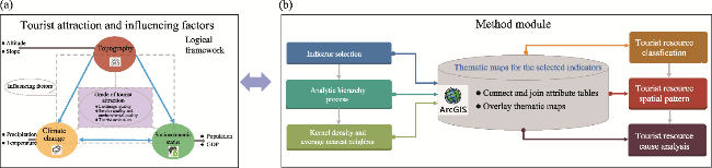
Figure 1 Logical framework for quantifying the spatial structure of tourist attractions

2.2 Indicator development procedure

The classification of tourist attractions includes the following: landscape, service, and environmental quality and tourist evaluation. The indicators were obtained from previous studies, expert consultations, and tourism management studies. The analytic hierarchy process (AHP) method was used to establish an indicator, with the weighting of each evaluation element assigned by expert judgment. Twenty experts in relevant fields were invited, among whom sixteen agreed to take part in the process of selecting indicators. The AHP method provides a way to systematise the complexities of grading tourist attractions, is easy to operate, and can incorporate the opinions of various stakeholders. The definitive 19 indicators and their respective weights were ascertained (Figure 2). After summarising the scores of the various indicators, tourist attractions were graded as shown in Table 1.
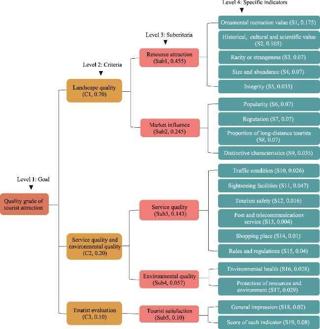
Figure 2 The classification index system of tourist attractions based on AHP
Table 1 Standard of rating for quality of tourist attractions
Grade Landscape
quality
Service and
environmental quality
Tourist
evaluation
5A ≥90 ≥95 ≥90
4A [80, 90) [85, 95) [80, 90)
3A [70, 80) [75, 85) [70, 80)
2A [60, 70) [60, 75) [60, 70)
1A [50, 60) [50, 60) [50, 60)

Note: This table refers to the national standards for the classification and evaluation of the quality of China’s tourist attractions (GB/T17775-2024).

2.3 Data sources

China has five widely distributed terrains—plateaus, mountains, hills, basins, and plains—and five climates—tropical monsoon, subtropical monsoon, temperate monsoon, temperate continental, and highland mountains. This diverse geographical environment has engendered a wealth of natural and anthropogenic tourism assets, such as the Great Wall, the Palace Museum, and Jiuzhaigou. Since the 1980s, China has become one of the world’s most important tourist destinations owing to the rapid growth in its tourism (Wen 1998). Therefore, we conducted a case study in China to demonstrate the proposed method’s efficacy.
We obtained basic information about China’s scenic spots through domestic authoritative tourism websites, literature reviews, and surveys. Elevation and slope were extracted using a digital elevation model (DEM) from the Global Multi-resolution Tree in Elevation Data. Monthly mean temperature and precipitation data were downloaded from the National Tibetan Plateau Science Data Center. Based on the relationship between nighttime lighting data and the GDP, we produced rasterised GDP data. Population distribution data were obtained from the World Pop website. The collected data did not include data for the three Chinese provinces (regions) of Hong Kong, Macao, and Taiwan.

2.4 Methods of data analysis

2.4.1 Average nearest neighbour

The average nearest neighbour method is widely used to analyse the spatial patterns of geographical elements, and we used this method to measure the distribution characteristics of tourist attractions (Clark and Evans, 1954). First, the distance between the central point of each tourist attraction and that of its nearest tourist attraction was measured. Subsequently, the average of all nearest neighbour distances was calculated. If the average distance was less than that in the assumed random distribution, tourist attractions were judged to be clustered. If the average distance was greater than that in the assumed random distribution, tourist attractions were judged to be dispersed. The mean nearest neighbour ratio (ANN) is used as a key parameter to quantify spatial relationships and is calculated by dividing the calculated mean distance by the expected mean distance, as follows:
$A N N=\frac{\bar{D}_{o}}{\bar{D}_{e}}=\frac{\frac{1}{n} \sum_{i=1}^{n} d_{i}}{0.5 / \sqrt{n / a}}$
where D¯o is the average distance between a tourist attraction and its nearest neighbour;D¯e is the average distance of the random distribution between the tourist attractions;diis the distance between scenic spot i and its nearest scenic spot; n is the number of scenic spots; and a is the area of the envelope of all scenic spots. If ANN was greater than 1, the distribution was random. If ANN is less than 1, it indicates a clustered distribution. The calculation was performed using the ArcGIS spatial statistics tool.

2.4.2 Kernel density analysis

We used kernel density analysis to express the high-density, low-density, and cluster characteristics of the distribution of tourist attractions. Kernel density analysis is a nonparametric statistical method used to estimate the data distribution that can reflect the visual state of discrete measured values in a continuous region (Silverman 2018). The kernel density function is expressed as follows, and ArcGIS software was used to show this function in the form of images:
fnx=1nhi=1nkxxih
where k is the weight function of the kernel; and h is the bandwidth—the width of the surface with x as the origin in space; x-xi is the distance between the density estimate points x and xi.

2.4.3 Statistical approach

To compare the differences in elevation, slope, temperature, precipitation, population, and GDP among different levels of scenic spots, we used the Quartile function in Excel to calculate the maximum and minimum values, upper and lower quartile, median and average values of these factors, and their change rates in the past few decades. Subsequently, we presented the results with a box chart. Additionally, a spatial Lorentz curve was used to describe the balanced distribution of the cumulative percentage of tourist attractions among different regions.

3 Results

3.1 Spatial characteristics of tourist attractions

Based on existing tourism data in China, a total of 13603 Class A tourist attractions in 31 provinces were statistically analyzed including 315 Class 5A, 4179 Class 4A, 6931 Class 3A, 2091 Class 2A, and 87 Class 1A scenic spots. The number of scenic spots was dominated by Grades 4A and 3A scenic spots, both accounting for 80.9%. Zhejiang Province had the highest number of scenic spots at 1322, and Hainan Province had the lowest at 81. Zhejiang Province had the highest number of 5A scenic spots, at 34 (Figure 3). The spatial Lorentz curve shows that among the 31 provinces surveyed, eight provinces, including Hainan, Tianjin, and Ningxia, had a cumulative percentage of less than 10%, and Guangxi, Jiangsu, and Sichuan had a high cumulative percentage (>70%) (Figure 4).
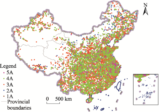
Figure 3 Spatial distribution of tourist attractions at each level (1A-5A)
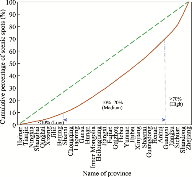
Figure 4 The spatial Lorentz curve of the distribution of scenic spots in 31 provinces

Note: The green line is the theoretical equality of spatial distribution. The red line represents the cumulative percentage of scenic spots in each province. The blue line is a subjective grading of cumulative percentages for comparison purposes.

The results of the average nearest neighbour and kernel density analyses in ArcGIS show the spatial aggregation state of the scenic spots. The nearest proximity ratio was less than 1, and the Z-score corresponded to the blue area in the figure, indicating a significant clustering spatial pattern of scenic spots (Figure 5a). The nuclear density values indicate that scenic spots are mainly clustered in eastern and southern China. The red and yellow areas show four important clustering centres along the eastern seaboard (Figure 5b).
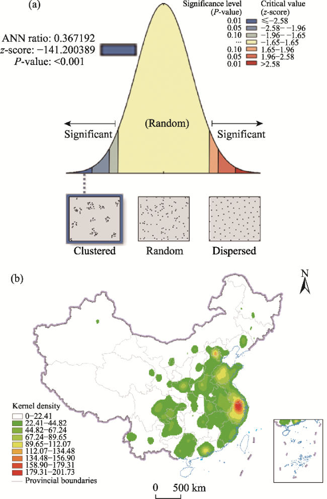
Figure 5 Results of average nearest neighbor and kernel density (a) average nearest neighbor calculation; (b) kernel density value of spatial structure of tourist attraction

Note:ANN ratio is mean nearest neighbor ratio. z-score is used to test the statistical significance of spatial autocorrelation analysis, where negative z-score represents agglomeration and positive z-score represents divergence. p values are probability values.

3.2 Effects of natural environment on tourist attractions

According to the statistics on the distribution of scenic spots by altitude, scenic spots were mainly distributed in areas below 200 m, accounting for 51.46% of the total number of scenic spots, and the number of scenic spots at 200-500 m, 500-1000 m, and 1000-3500 m altitudes accounts for 17.64%, 12.64%, and 16.86%, respectively, of the total number of scenic spots. The number of scenic spots in alpine areas above 3500 m above sea level was the lowest at only 190, accounting for 1.4% of the total scenic spots (Figure 6a). The statistical results of the different gradients showed that all types of scenic spots were mainly located in areas with gradients less than 15°, accounting for 95.10% of the total number of scenic spots. The number of regional scenic spots with slopes less than 5° accounted for 74.88% of the total number of scenic spots, and the number of regional scenic spots with slopes between 5° and 15° accounted for 20.21% of the total number of scenic spots (Figure 6b).
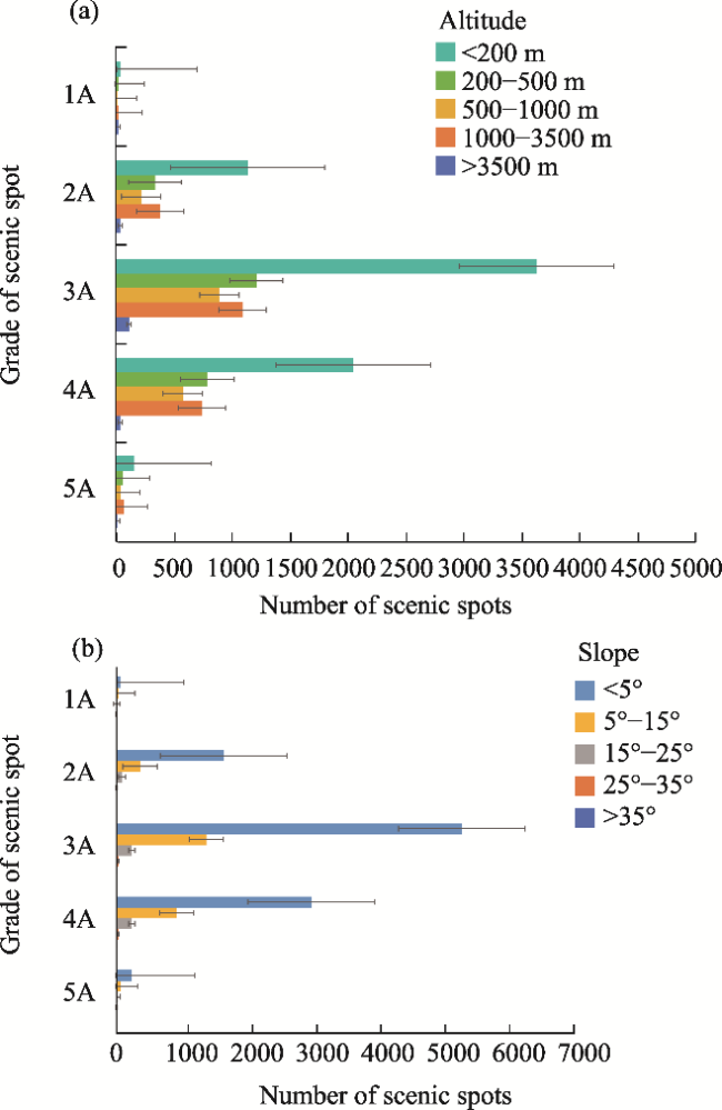
Figure 6 Elevation and slope distribution characteristics of spatial structure of tourist attractions (a) elevation; (b) slope
The analysis of temperature and precipitation from 1960 to 2022 showed that scenic spots 5A, 4A, and 3A had similar average temperatures and precipitation. Scenic spots 1A and 2A have relatively low temperatures and less precipitation but high temperature variability (Figure 7). There was little difference in precipitation variability among the five scenic spot levels (Figure 8). Notably, the lower-grade 1A and 2A scenic spots are mainly distributed in areas with low temperature and little precipitation. The higher-grade 5A, 4A, and 3A scenic spots had similar climatic characteristics because of their more concentrated distribution areas.
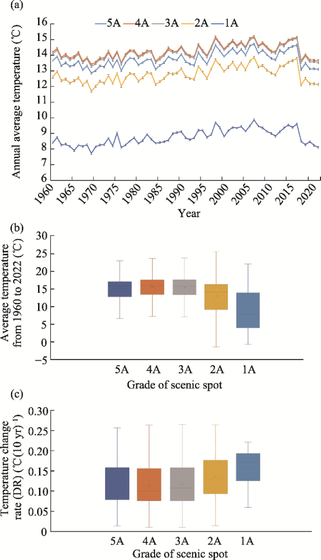
Figure 7 Temperature characteristics of different levels of tourist attractions (a) average temperature; (b) average temperature of different levels of scenic spots; (c) temperature change rate of different levels of scenic spots
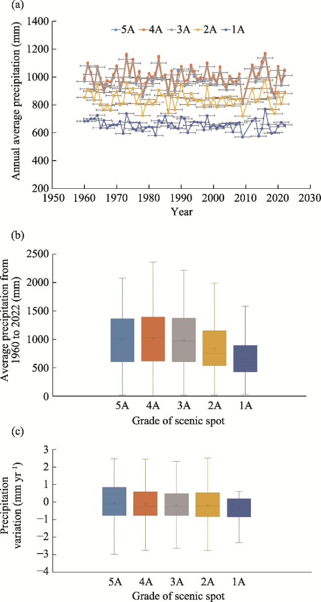
Figure 8 Precipitation characteristics of different levels of tourist attractions (a) interannual characteristics of mean precipitation; (b) the average precipitation of different levels of scenic spots; (c) precipitation variation of different scenic spots

3.3 Human activities and distribution of tourist attractions

In the past 20 years, the GDP and population density show that the 5A scenic spots have a high GDP, population density, and growth rate. The GDP and population density of the 2A scenic spot were second only to those of the 5A scenic spot (Figure 9). The growth rate of the population den-sity in all scenic spots was low, and there was no significant difference in the growth rate between the different levels (Figure 9). Figure 10 shows the geographical division line based on demographic and economic factors. The proportions of population in the southeast and northwest regions were 94% and 6%, respectively, and the proportions of GDP were 95% and 5%, respectively. In the southeastern region, A-level scenic spots or above accounted for approximately 60% of the total scenic spots. The layout of tourist attractions is closely related to the population distribution and economic development in space.
Figure 9 GDP and population density of different levels of scenic spots (a) average GDP; (b) GDP variation; (c) population density; (d) population density variation
Figure 10 Spatial structure of tourist attractions based on geographical dividing lines

4 Discussion

4.1 Indicators and weights

Tourist attractions have the characteristics of many types, wide distribution, different scales, and concrete and abstract coexistence; therefore, it is complicated to classify them. However, the country or region to formulate tourism planning and management must be based on classification and grading evaluation (Biagi and Pearce, 2010; Budeanu et al., 2016). Owing to the lack of universal evaluation criteria, many studies have established an evaluation index system for a certain type or region of tourism resource and adopted an expert scoring method to assign different weights (Kittidachanupap et al., 2014; Asmelash and Kumar, 2019). To reduce the uncertainty and eliminate bias, we solved the problem in three ways. First, we used the AHP—a qualitative and quantitative decision analysis method used to solve multiobjective complex problems. Considering the complexity of the evaluation objects, the hierarchical model we constructed adds a sub-criterion layer based on the traditional target, criterion, and index scheme layers. The second was to increase the number of experts when there was a significant difference in the scores for a certain indicator. Third, experts were selected from various fields, such as tourism, resources, and management. Furthermore, it is essential to develop specialized indicator systems for various categories of tourism assets and distinct administrative territories in the future.

4.2 Classification and influencing factors

Terrain and climate shape most natural landscapes (Krummel et al., 1987). China’s terrain is roughly divided into three steps according to elevation. The second and third stairs at low altitudes are concentrated areas of tourist attractions above Grade A. The Tibetan Plateau, located in the first step, has an average altitude of > 4500 m. Owing to the cold climate, lack of oxygen, and inconvenient transportation, the distribution of scenic spots above Class A is low. However, the region has unique natural landscapes, such as mountains, glaciers, and plateau lakes, with high tourism value, attraction, and global attention. After weighing the conditions of tourism security and the economic and social factors, our classification appears to weaken the value of tourist attractions in the region.

4.3 Spatial structure

Space is defined in geography as the ‘geometry’ or ‘motion’ of the earth’s surface. Distance, proximity, and topological relations are the key parameters for characterising spatial structure, and their logical relations and theoretical frameworks are usually reflected in drawing (Bunge, 1979). This study was based on spatial topological analysis and graph theory. The developed SSTA shows the geographical patterns of tourist attractions and provides a scientific method for the spatial selection of tourism planning and management. Although we focused on the spatial structure of tourist destinations, the analysis of the spatial characteristics of tourists and tourism is insufficient. In the future, it is imperative that we intensify our research efforts on tourist source markets, their distribution patterns, and the potential impact of climate change. Furthermore, delving into the study of dynamic spatial structures across various time periods will undoubtedly enhance our comprehension and insights.

5 Conclusions

The formation of the spatial distribution pattern of tourist attractions is a complex and long-term process, which is affected by the quality of tourist attractions, security conditions, and service levels and is closely related to the natural environment, economic status, and social development of tourist attractions. This study measured the spatial structure of tourist attractions in China and its influencing factors, which is realised by combining the grade evaluation of tourist attractions, analysis of natural and socioeconomic factors, and GIS. In terms of scientific contributions, this study provides new insights into the spatial distribution of tourist attractions and their formation reasons. The scenic spot classification method, with four levels and 29 indicators, provides an innovative way to combine hierarchical analysis with target decision-making. This method allowsvarious evaluation indicators and monitoring data to be incorporated into a GIS, which can achieve intuitive visualisation and easy real-time data updates. This method was used to evaluate the spatial characteristics of the main scenic spots in China and to compare the topographic differences, climate changes, and social and economic dynamics of the scenic spots, providing a new idea for the sustainable management of tourist attractions.
[1]
Alcalá-Ordóñez A, Brida J G, Cardenas-García P J, et al. 2023. Tourism as an instrument of economic growth: Empirical exploration at the regional level in Spain. Natural Resources Forum, 47(2): 187-205.

[2]
Aminu M, Ludin A N B, Matori A N, et al. 2013. A spatial decision support system (SDSS) for sustainable tourism planning in Johor Ramsar sites, Malaysia. Environmental Earth Sciences, 70(3): 1113-1124.

[3]
Arya V, Auruskeviciene V, Agarwal S, et al. 2024. Let us take a walk to the sustainable tourism practices: A qualitative study through the lens of tourism experts. Environmental Science and Pollution Research, 31(5): 7890-7905.

[4]
Asmelash A G, Kumar S. 2019. Assessing progress of tourism sustainability: Developing and validating sustainability indicators. Tourism Management, 71: 67-83.

[5]
Bafaluy D, Amengual A, Romero R, et al. 2014. Present and future climate resources for various types of tourism in the Bay of Palma, Spain. Regional Environmental Change, 14(5): 1995-2006.

[6]
Balbi S, Giupponi C, Perez P, et al. 2013. A spatial agent-based model for assessing strategies of adaptation to climate and tourism demand changes in an alpine tourism destination. Environmental Modelling & Software, 45: 29-51.

[7]
Barbero J, Zofío J L. 2016. The multiregional core-periphery model: The role of the spatial topology. Networks & Spatial Economics, 16(2): 469-496.

[8]
Baum J, Cumming G S, De Vos A. 2017. Understanding spatial variation in the drivers of nature-based tourism and their influence on the sustainability of private land conservation. Ecological Economics, 140: 225-234.

[9]
Biagi B, Pearce P. 2010. The evolution of tourism demand and supply: A regional policy study. International Journal of Tourism Policy, 3(3): 237-256.

[10]
Bowen D. 2022. Contemporary tourist behaviour: Yourself and others as tourists. Oxford, UK: CABI Digital Library.

[11]
Budeanu A, Miller G, Moscardo G, et al. 2016. Sustainable tourism, progress, challenges and opportunities: An introduction. Journal of Cleaner Production, 111: 285-294.

[12]
Bunge W. 1979. Perspective on theoretical geography. Annals of the Association of American Geographers, 69(1): 169-174.

[13]
Carrillo M, Jorge J M. 2017. Multidimensional analysis of regional tourism sustainability in Spain. Ecological Economics, 140: 89-98.

[14]
Chang M Y, Hsu Y S, Chen H S. 2021. Choice experiment method for sustainable tourism in theme parks. Sustainability, 13(13): 7146. DOI: 10.3390/su13137146.

[15]
Chen N, Li H, Wang L. 2009. A GIS-based approach for mapping direct use value of ecosystem services at a county scale: Management implications. Ecological Economics, 68(11): 2768-2776.

[16]
Clark P J, Evans F C. 1954. Distance to nearest neighbor as a measure of spatial relationships in populations. Ecology, 35(4): 445-453.

[17]
Deng J, King B, Bauer T. 2002. Evaluating natural attractions for tourism. Annals of Tourism Research, 29(2): 422-438.

[18]
Dong Y X, Zhou B G, Yang G H, et al. 2023. A novel model for tourism demand forecasting with spatial-temporal feature enhancement and image-driven method. Neurocomputing, 556: 126-141.

[19]
Douglas P. 1995. Tourist development:A geographical analysis. Jalan, Singapore: Longman Press.

[20]
Firdaus N M, Chahyati D, Fanany M I. 2018. Tourist attractions classification using ResNet. International Conference on Advanced Computer Science and Information Systems. Yogyakarta, Indonesia: IEEE Computer Society.

[21]
Gidebo H B. 2021. Factors determining international tourist flow to tourism destinations: A systematic review. Journal of Hospitality Management and Tourism, 12(1): 9-17.

[22]
Guo X L, Wu B H, Liu L, et al. 2000. Study on the tourist resources classification system and types evaluation in China. Acta Geographica Sinica, 55(3): 294-301. (in Chinese)

DOI

[23]
Hu Q, Xiang L Q, Lin A W, et al. 2024. Exploring the spatial configuration of tourism resources through ecosystem services and ethnic minority villages. Ecological Informatics, 79: 102-121.

[24]
Joshi O, Poudyal N C, Larson L R. 2017. The influence of sociopolitical, natural, and cultural factors on international tourism growth: A cross-country panel analysis. Environment, Development and Sustainability, 19(3): 825-838.

[25]
Kim J, Kang Y. 2022. Automatic classification of photos by tourist attractions using deep learning model and image feature vector clustering. ISPRS International Journal of Geo-Information, 11(4): 245-262.

[26]
Kim Y J, Lee D K, Kim C K. 2020. Spatial tradeoff between biodiversity and nature-based tourism: Considering mobile phone-driven visitation pattern. Global Ecology and Conservation, 21: 1-13.

[27]
Kittidachanupap N, Angsakun J, Angsakun T. 2014. A comparison of expert-based and tourist-based methods for tourist attraction ranking. International Information Institute (Tokyo) Information, 17(6): 1991-1998.

[28]
Könnyid L, Váradi Z, Nagy Z, et al. 2022. The changes in the demographic characteristics and spatial structure of tourism demand in the west Balaton region’s spa cities. Sustainability, 14(17): 10531. DOI: 10.3390/su141710531.

[29]
Krummel J, Gardner R, Sugihara G, et al. 1987. Landscape patterns in a disturbed environment. Oikos, 48(3): 321-324.

[30]
Lin C H, Kuo B Z L. 2016. The behavioral consequences of tourist experience. Tourism Management Perspectives, 18: 84-91.

[31]
Machairas A, Hovardas T. 2005. Determining visitors’ dispositions toward the designation of a Greek national park. Environmental Management, 36(1): 73-88.

PMID

[32]
Mangubhai S, Sykes H, Manley M, et al. 2020. Contributions of tourism-based marine conservation agreements to natural resource management in Fiji. Ecological Economics, 171: 106607. DOI: 10.1016/j.ecolecon.106607.

[33]
Mazanec J. 1983. Tourist behavior model building: A causal approach. The Tourist Review, 38(1): 9-19.

[34]
McKercher B. 2017. Do attractions attract tourists? A framework to assess the importance of attractions in driving demand. International Journal of Tourism Research, 19(1): 120-125.

[35]
McKercher B, Lau G. 2008. Movement patterns of tourists within a destination. Tourism Geographies, 10(3): 355-374.

[36]
Novianti S, Fauzi C, Suhartanto D. 2020. Spatial analysis of tourist dispersal and mobility for tourism destination planning and development:A case study of Great Ocean Road region, Australia. IOP Conference Series:Materials Science and Engineering. Singapore: Institute of Physics.

[37]
Richards G. 2002. Tourism attraction systems: Exploring cultural behavior. Annals of Tourism Research, 29(4): 1048-1064.

[38]
Roman M, Roman M, Niedziólka A. 2020. Spatial diversity of tourism in the countries of the European Union. Sustainability, 12(7): 2713. DOI: 10.3390/su12072713.

[39]
Sano K, Sano H, Yashima Y, et al. 2024. The effects of temporal distance and post type on tourists’ responses to destination marketing organizations’ social media marketing. Tourism Management, 101: 104844. DOI: 10.1016/j.tourman.2023.104844.

[40]
Sarrión-Gavilán M D, Benítez-Márquez M D, Mora-Rangel E O. 2015. Spatial distribution of tourism supply in Andalusia. Tourism Management Perspectives, 15: 29-45.

[41]
Scott D, McBoyle G, Schwartzentruber M. 2004. Climate change and the distribution of climatic resources for tourism in North America. Climate Research, 27(2): 105-117.

[42]
Silverman B W. 2018. Density estimation for statistics and data analysis. New York, USA: Routledge.

[43]
Tsilimigkas G, Rempis N. 2021. Spatial planning framework, a challenge for marine tourism development: Location of diving parks on Rhodes island, Greece. Environment Development and Sustainability, 23(10): 15240-15265.

DOI

[44]
Ullah A, Raza K, Mehmood U. 2023. The impact of economic growth, tourism, natural resources, technological innovation on carbon dioxide emission: Evidence from BRICS countries. Environmental Science and Pollution Research, 30(15): 42854-42871.

[45]
Wang C, Xu L L, Huang M L, et al. 2022. Research on the evolution of spatial network structure of tourism eco-efficiency and its influencing factors in China’s provinces based on carbon emission accounting. Plos One, 17(9): e0272667. DOI: 10.1371/journal.pone.0272667.

[46]
Wen J. 1998. Evaluation of tourism and tourist resources in China: Existing methods and their limitations. International Journal of Social Economics, 25(2/3/4): 467-485.

[47]
Zhan H B, Liu S F, Shao Q L. 2015. Evaluation of eco-tourism resources of forest nature reserves based on Grey Cluster Model. Journal of Grey System, 27(3): 249-258.

Outlines

/