
Journal of Resources and Ecology >
The Impact and Mechanism Analysis of Digital Inclusive Finance on Urban Green Development
|
LIU Yunqin, E-mail: yunqin0626@126.com |
Received date: 2024-04-03
Accepted date: 2024-09-01
Online published: 2025-08-05
Supported by
The Nanchang Social Science Planning Project(YJ202329)
The Humanities and Social Science Project of Nanchang Institute of Science & Technology(NGRW-22-02)
Based on the panel data of Chinese cities during 2013 and 2021, this study establishes a panel fixed-effect model and a panel threshold model to empirically investigate the effect of digital inclusive finance on urban green development, as well as the mechanism, threshold characteristics and heterogeneity. The study reveals the following four points: (1) Digital inclusive finance can significantly drive urban green development, whose coverage breadth has more prominent promotional effect on urban green development compared to the usage depth and the digitization level. (2) In terms of the acting mechanism, the current effect of digital inclusive finance on urban green development is mainly achieved through promoting economic development and environmental protection, while its promotion effect on social progress is not yet significant. (3) The impact of digital inclusive finance on urban green development varies depending on the agglomeration degree of urban digital economy and its geographical location. In non-agglomeration areas of digital economy and western regions, the promotion effect of digital inclusive finance on urban green development is more obvious. (4) The promotion effect of digital inclusive finance on urban green development exhibits non-linear characteristics with different levels of urban economic development and digital inclusive finance development.
LIU Yunqin , JIANG Tingyao . The Impact and Mechanism Analysis of Digital Inclusive Finance on Urban Green Development[J]. Journal of Resources and Ecology, 2025 , 16(4) : 1052 -1063 . DOI: 10.5814/j.issn.1674-764x.2025.04.011
Table 1 Comprehensive index of urban green development |
| Primary index | Dimensions | Specific indicators | Indicator attribute |
|---|---|---|---|
| Urban green development (Gde) | Economic development (Ed) | Per capita GDP | + |
| GDP growth rate | + | ||
| Labor productivity | + | ||
| Proportion of tertiary industry | + | ||
| Government technology expenditure | + | ||
| Environmental protection (Ep) | Electricity consumption per unit of GDP | - | |
| Total water supply per unit GDP | - | ||
| Construction land per unit GDP | - | ||
| Utilization rate of general industrial solid waste | + | ||
| Centralized processing rate of sewage | + | ||
| Harmless treatment rate of domestic garbage | + | ||
| Removal rate of SO2 | + | ||
| Social progress (Sp) | The rate of green coverage in built up areas | + | |
| Bus ownership per 10000 people | + | ||
| Public library collection per 100 people | + | ||
| Per capita urban road area | + | ||
| Per capita number of beds in hospital and medical institutions | + | ||
| Internet penetration rate | + |
Table 2 Descriptive statistical results of main variables |
| Variables | Observations | Mean | Standard deviation | Min | Max | |
|---|---|---|---|---|---|---|
| Explained variable | Gde | 2556 | 1.780 | 0.775 | 0.004 | 7.936 |
| Explanatory variables | Difi | 2556 | 5.311 | 0.275 | 4.475 | 5.885 |
| coverage_breadth | 2556 | 5.259 | 0.307 | 4.190 | 5.918 | |
| usage_depth | 2556 | 5.270 | 0.314 | 4.254 | 5.870 | |
| digitization_level | 2556 | 5.501 | 0.230 | 4.560 | 6.365 | |
Control variables | ind | 2556 | 44.139 | 11.173 | 11.040 | 82.230 |
| fdi | 2556 | 10.111 | 1.933 | 2.708 | 14.941 | |
| env | 2556 | 80.068 | 20.895 | 0.340 | 101.907 | |
| inf | 2556 | 0.031 | 0.040 | 0.002 | 0.486 | |
| fin | 2556 | 1.104 | 0.632 | 0.118 | 9.622 | |
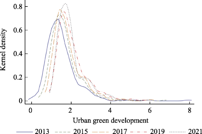
Figure 1 Time-series dynamic evolutionary characteristics of the Gde level |
Table 3 Benchmark regression results |
| Variables | Gde | ||||
|---|---|---|---|---|---|
| (1) | (2) | (3) | (4) | (5) | |
| Difi | 0.515*** | 0.511** | |||
| (0.177) | (0.202) | ||||
| coverage_breadth | 0.527*** | ||||
| (0.0364) | |||||
| usage_depth | 0.308*** | ||||
| (0.0311) | |||||
| digitization_level | 0.304*** | ||||
| (0.0363) | |||||
| ind | −0.0041*** | −0.0035** | −0.0081*** | −0.0097*** | |
| (0.0014) | (0.0015) | (0.0015) | (0.0014) | ||
| fdi | −0.0093 | −0.0117 | −0.0101 | −0.0116 | |
| (0.0087) | (0.0092) | (0.00942) | (0.0095) | ||
| env | 0.001* | 0.0007 | 0.0011* | 0.0006 | |
| (0.0005) | (0.0006) | (0.0006) | (0.0006) | ||
| inf | 0.809*** | 0.0582 | 0.389** | 0.443** | |
| (0.192) | (0.175) | (0.177) | (0.178) | ||
| fin | 0.0409* | 0.0382* | 0.0707*** | 0.0869*** | |
| (0.0218) | (0.0230) | (0.0235) | (0.0234) | ||
| Constant | −0.969 | −0.905 | −1.037*** | 0.200 | 0.230 |
| (0.857) | (0.988) | (0.251) | (0.231) | (0.259) | |
| City fixed effect | Yes | Yes | Yes | Yes | Yes |
| Year fixed effect | Yes | Yes | Yes | Yes | Yes |
| Obs. | 2556 | 2556 | 2556 | 2556 | 2556 |
| R2 | 0.336 | 0.346 | 0.254 | 0.214 | 0.203 |
| Number of id | 284 | 284 | 284 | 284 | 284 |
Note: *, ** and *** indicate statistical significance at the 10%, 5% and 1% levels, respectively. Standard errors are in parentheses. The same below. |
Table 4 Instrumental regression results |
| Variables | (1) | (2) | (3) | (4) |
|---|---|---|---|---|
| Difi | Gde | Difi | Gde | |
| Difi | 3.3165*** (0.7294) | 0.5867*** (0.0502) | ||
| iv1 | 0.0054*** (0.0010) | |||
| iv2 | 0.8207*** (0.0068) | |||
| Constant | 1.157*** (0.024) | −1.692*** (0.175) | 1.053*** (0.0382) | −1.4316*** (0.3317) |
| Controls | Yes | Yes | Yes | Yes |
| City fixed effect | Yes | Yes | Yes | Yes |
| Year fixed effect | Yes | Yes | Yes | Yes |
| K-P LM statistics | 87.46*** | 146.55*** | ||
| K-P Wald rk F statistics | 32.38 | 369.24 | ||
| Obs. | 2556 | 2556 | 2272 | 2272 |
| R2 | 0.1926 | 0.0374 | 0.2010 | 0.1947 |
Table 5 Robustness test |
| Variables | (1) Replacing the core explanatory variable | (2) Excluding the municipalities | (3) Winsorize | (4) GLS |
|---|---|---|---|---|
| Difi | 0.4160* | 0.542*** | 0.371* | 0.6940*** |
| (0.2126) | (0.205) | (0.192) | (0.0267) | |
| Constant | −0.4074 | −1.059 | −0.313 | −3.688*** |
| (1.0445) | (1.001) | (0.938) | (0.1443) | |
| Controls | Yes | Yes | Yes | Yes |
| City fixed effect | Yes | Yes | Yes | Yes |
| Year fixed effcet | Yes | Yes | Yes | Yes |
| Obs. | 2272 | 2520 | 2556 | 2556 |
| R2 | 0.1633 | 0.348 | 0.399 | 0.190 |
Table 6 Heterogeneity analysis |
| Variables | Gde | ||||
|---|---|---|---|---|---|
| (1) Eastern | (2) Central | (3) Western | (4) Digital economy agglomeration area | (5) Digital economy non-agglomeration area | |
| Difi | 0.408*** | 0.476*** | 0.635*** | 0.336*** | 0.548*** |
| (0.0824) | (0.0429) | (0.0727) | (0.122) | (0.0374) | |
| Constant | 0.108 | −1.082*** | −1.747*** | −0.675 | −1.290*** |
| (0.600) | (0.294) | (0.484) | (0.971) | (0.256) | |
| Controls | Yes | Yes | Yes | Yes | Yes |
| City fixed | Yes | Yes | Yes | Yes | Yes |
| Year fixed | Yes | Yes | Yes | Yes | Yes |
| Obs. | 900 | 882 | 774 | 567 | 1989 |
| R2 | 0.131 | 0.353 | 0.347 | 0.160 | 0.308 |
Table 7 Mechanism test: Full sample |
| Variables | (1) Economic development (Ed) | (2) Environmental protection (Ep) | (3) Social progress (Sd) |
|---|---|---|---|
| Difi | 0.0442*** | 0.162*** | 0.0028 |
| (0.0035) | (0.0081) | (0.0028) | |
| Constant | -0.203*** | 1.025*** | 0.0722*** |
| (0.0241) | (0.0561) | (0.0197) | |
| Controls | Yes | Yes | Yes |
| City fixed effect | Yes | Yes | Yes |
| Year fixed effect | Yes | Yes | Yes |
| Obs. | 2556 | 2556 | 2556 |
| R2 | 0.165 | 0.414 | 0.010 |
Table 8 Mechanism test: Regional division |
| Variables | Eastern region | Central region | Western region | ||||||
|---|---|---|---|---|---|---|---|---|---|
| Ed | Ep | Sd | Ed | Ep | Sd | Ed | Ep | Sd | |
| Difi | 0.0785*** | 0.135*** | -0.0062 | 0.0372*** | 0.185*** | 0.0035 | 0.0122*** | 0.155*** | 0.0177*** |
| (0.0092) | (0.0139) | (0.0064) | (0.0043) | (0.0138) | (0.0028) | (0.0012) | (0.0151) | (0.0055) | |
| Constant | -0.354*** | 1.023*** | 0.162*** | -0.217*** | 1.026*** | 0.0517*** | -0.042*** | 0.989*** | -0.0137 |
| (0.067) | (0.101) | (0.0466) | (0.0294) | (0.0947) | (0.0190) | (0.0077) | (0.101) | (0.0365) | |
| Controls | Yes | Yes | Yes | Yes | Yes | Yes | Yes | Yes | Yes |
| City fixed | Yes | Yes | Yes | Yes | Yes | Yes | Yes | Yes | Yes |
| Year fixed | Yes | Yes | Yes | Yes | Yes | Yes | Yes | Yes | Yes |
| Obs. | 900 | 900 | 900 | 882 | 882 | 882 | 774 | 774 | 774 |
| R2 | 0.160 | 0.387 | 0.016 | 0.369 | 0.444 | 0.054 | 0.406 | 0.438 | 0.065 |
Table 9 Threshold effect test results |
| Threshold variables | Threshold type | Threshold value | F-value | P-value | Bootstrap | Critical value | ||
|---|---|---|---|---|---|---|---|---|
| 10% | 5% | 1% | ||||||
| pgdp | Single threshold | 14.9277 | 30.38 | 0.0100 | 300 | 16.8656 | 18.9587 | 27.9243 |
| Double threshold | - | 24.35 | 0.1367 | 300 | 0.000 | 0.000 | 0.000 | |
| Difi | Single threshold | 5.3399 | 54.84 | 0.0367 | 300 | 48.2504 | 51.8629 | 62.9351 |
| Double threshold | 5.1452, 5.6732 | 51.37 | <0.001 | 300 | 32.5538 | 36.5643 | 45.1225 | |
| Triple threshold | - | 45.21 | 0.6400 | 300 | 0.000 | 0.000 | 0.000 | |
Table 10 Threshold effect regression results |
| Variables | Gde | |
|---|---|---|
| Threshold_pgdp (1) | Threshold_Difi (2) | |
| Threshold1 | 0.4773*** (7.50) | 0.7441*** (7.96) |
| Threshold2 | 0.5368*** (9.58) | 0.8170*** (10.02) |
| Threshold3 | - | 0.8544*** (10.02) |
| Controls | Yes | Yes |
| City fixed effect | Yes | Yes |
| Year fixed effect | Yes | Yes |
| Obs. | 2556 | 2556 |
| R2 | 0.2738 | 0.1811 |
Note: The T values are in parentheses. |
| [1] |
|
| [2] |
|
| [3] |
|
| [4] |
|
| [5] |
|
| [6] |
|
| [7] |
|
| [8] |
|
| [9] |
|
| [10] |
|
| [11] |
|
| [12] |
|
| [13] |
|
| [14] |
|
| [15] |
|
| [16] |
|
| [17] |
|
| [18] |
|
| [19] |
|
| [20] |
|
| [21] |
|
| [22] |
|
| [23] |
|
| [24] |
|
| [25] |
|
| [26] |
|
| [27] |
|
| [28] |
|
| [29] |
|
| [30] |
|
| [31] |
|
| [32] |
|
| [33] |
|
| [34] |
|
| [35] |
|
| [36] |
|
| [37] |
|
| [38] |
|
/
| 〈 |
|
〉 |