
Journal of Resources and Ecology >
The Spatio-temporal Characteristics of Shanghai Tourist Flow Network Based on Change Point Detection
|
XIA Shuang, E-mail: 307236628@qq.com |
Received date: 2024-04-03
Accepted date: 2024-08-01
Online published: 2025-03-28
Supported by
The Key Project of National Natural Science Foundation of China(42130510)
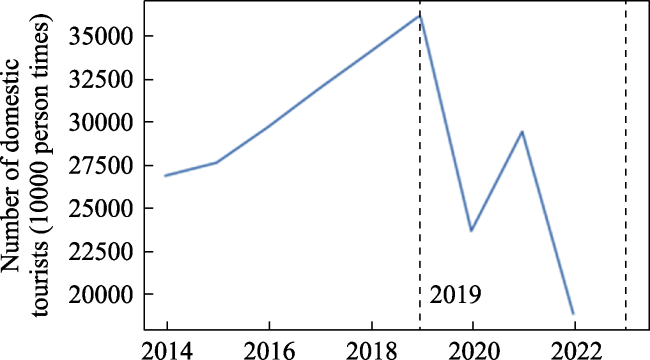
Taking Shanghai as an example, this study obtained the online travel notes data from Xiaohongshu and Qunar in the past 10 years to construct the Shanghai tourist flow network (STFN) and used the methods of change point detection (CPD) and complex network analysis (CNA) to reveal the spatial structure characteristics of Shanghai tourism flow and the dynamic evolution process of STFN. The results showed that: (1) In the past 10 years, Shanghai tourist market had experienced a process of evolution from stable and orderly to short-term fluctuation and then gradual recovery, and the year of 2019 was the turning point of tourist flow network evolution. (2) The small-world and approximate scale-free characteristics of STFN were verified, and the network changed from disassortative to temporary assortative, showing a development trend of external expansion and internal separation. (3) While the centrality indicators of tourist flow network remained stable as a whole, the attention to cultural nodes was also increasing with the emergence of new nodes; (4) In terms of spatial connection, new popular nodes emerged and the relationship between them and the surrounding nodes was strengthened; (5) The spatial pattern of tourist flow network presented an inverted “V” shape and gradually expanded to southwest and southeast, forming a network with core nodes as the center and radiating outward. At the same time, newly emerging nodes at the periphery had formed relatively independent clusters.
XIA Shuang , ZHANG Yao , FANG Tianhong . The Spatio-temporal Characteristics of Shanghai Tourist Flow Network Based on Change Point Detection[J]. Journal of Resources and Ecology, 2025 , 16(2) : 546 -557 . DOI: 10.5814/j.issn.1674-764x.2025.02.022
Table 1 Formulas and meanings of statistical indicators for complex networks |
| Indicators | Formula | Mathematical meaning | Concept definition |
|---|---|---|---|
| $\sigma $ | $\sigma =\frac{C}{Crand}\times \frac{Lrand}{L}$ | σ is a metric used to quantify the small-world characteristics of a network; C represents the actual clustering coefficient of the network; L represents the actual average shortest path length of the network; Crand represents the average clustering coefficient of a random graph with the same number of nodes and edges; Lrand represents the average shortest path length of a random graph with the same number of nodes and edges | Compare the network’s clustering and short path properties with the corresponding values in a random network. If σ is greater than 1, it indicates that the network exhibits small-world characteristics |
| $\omega $ | $\omega =\frac{Lr}{L}-\frac{C}{Cl}$ | ω is a metric used to quantify the small-world characteristics of a network; C and L represent the average shortest path length, Lr represents the average shortest path length of the equivalent random graph, and Cl represents the average clustering coefficient of the equivalent lattice graph | The clustering coefficient measures to what extent a network resembles a lattice or a random graph. $\omega $ close to 0 implies small-world characteristics |
| Degree | ${{k}_{i}}=\sum\limits_{j}{{{A}_{ij}}}$ | ki is the degree of node i; Aij indicates whether there is a connection between node i and node j, 1 if there is, or 0 if there is not | It represents the number of edges connecting a specific node to other nodes in a network, reflecting its centrality within the network |
| Degree of weighting | ${{k}_{wi}}=\sum\limits_{j}{{{w}_{ij}}}$ | kwi is the weighted degree of node i; wij represents the weight of the edge between node i and node j | It represents the weight of the edges between nodes in a network. It reflects the sum of the weights of the edges connecting a specific node to other nodes, indicating its connectivity strength within the network, i.e., its influence |
| Cumulative degree distribution | ${{P}_{cum}}(k)=P(K\ge k)$ | ${{P}_{cum}}(k)$ represents the proportion of nodes with degree at least k; K represents the degree of the node | Describe the probability distribution of node degrees in a network. It represents the cumulative probability of nodes with at least k connections in the network |
| Average clustering coefficient | ${{C}_{avg}}=\frac{1}{N}\sum\limits_{i=1}^{N}{{{C}_{i}}}$ | Cavg is the average clustering coefficient of the entire network; Ci represents the clustering coefficient of node i, and N represents the total number of nodes in the network | It reflects the aggregation of nodes in the network, which represents the network’s clustering tendency. |
| Average shortest path | ${{L}_{avg}}=\frac{1}{N(N-1)}\sum\limits_{i\ne j}{{{d}_{ij}}}$ | Lavg is the average shortest path length of the network; N represents the total number of nodes in the network; dij represents the shortest path length between node i and node j | It characterizes the average distance between any two nodes, reflecting the degree of separation among nodes in the network |
| Network density | $D=\frac{2\times L}{N\times (N-1)}$ | D represents the value of the network density; L represents the actual number of connections (edges) in the network, and N is the total number of nodes in the network | The greater the number of edges in the network, the denser the network is. |
| Network diameter | $D=\text{ma}{{\text{x}}_{i,j}}{{d}_{ij}}$ | D represents the value of the network diameter; dij represents the shortest path length between node i and node j | This indicates the maximum distance for information propagation within the network, which reflects the longest shortest path length between any two nodes in the network |
| The compatibility of node degrees | $r=\frac{\mathop{\sum }_{i,j}\left( {{A}_{ij}}-\frac{{{k}_{i}}{{k}_{j}}}{2m} \right)\delta ({{k}_{i}},{{k}_{j}})}{\mathop{\sum }_{i,j}\left( {{A}_{ij}}-\frac{{{k}_{i}}{{k}_{j}}}{2m} \right)(1-\delta ({{k}_{i}},{{k}_{j}}))}$ | r represents the compatibility of node degrees; Aij indicates whether there is a connection between node i and node j; ki represents the degree of node i ; m represents the number of edges in the network. δ (ki, kj) represents the Leopold Kronecker δ sign, which is 1 when k = kj and 0 otherwise | If assortativity is positive, it indicates that the network tends to connect nodes with similar degrees; conversely, it tends to connect nodes with different degrees |
| Near centrality | ${{C}_{i}}=\frac{1}{\frac{1}{N-1}\sum\limits_{j\ne i}{{{d}_{ij}}}}$ | Ci represents the near centrality value representing node i. N represents the total number of nodes in the network; dij represents the shortest path length between node i and node j | It measures the average distance from a node to other nodes in the network, indicating the centrality of the node within the network |
| Centrality of intermediate numbers | $CB(v)=\sum\limits_{\begin{smallmatrix} s\ne v,\ v\ne u \\ s,t\in V \\ s\ne t \end{smallmatrix}}{\frac{{{\sigma }_{st}}(v)}{{{\sigma }_{st}}}}$ | CB (ν) represents the betweenness centrality of node ν; σst represents the number of shortest paths from node s to node t; σst (ν) represents the number of shortest paths through node ν | It reflects the frequency with which a node lies on the shortest paths connecting other nodes in the network, thus indicating the node’s influence in information propagation within the network |
| Centrality of eigenvectors | $Ax=\lambda x$ | A represents the adjacency matrix of the network, representing the connections between nodes; x represents the eigenvector centrality of nodes; λ represents the eigenvalue corresponding to the eigenvector x | It is an index to measure the importance of nodes in a network, considering the connection strength between nodes and their neighbors |
Figure 1 Points of variation and stages of the Shanghai tourist market |
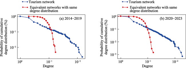
Figure 2 Scale-free characteristic metrics for the two-phase network |
Table 2 Table of indicators of small world characteristics for the two phases |
| Statistical stage | Average | Standard deviation | Coefficient of variation | |||
|---|---|---|---|---|---|---|
| σ | ω | σ | ω | σ | ω | |
| 2014-2019 | 1.150405 | -0.38931 | 0.051929 | 0.051414 | 0.04514 | -0.13207 |
| 2020-2023 | 2.315617 | -0.89681 | 0.091601 | 0.045524 | 0.039558 | -0.05076 |
Table 3 Statistics on the amount of network features in the two phases |
| Statistical stage | Number of nodes | Number of edges | Average clustering coefficient | Average shortest path | Network density | Network diameter |
|---|---|---|---|---|---|---|
| 2014-2019 | 411 | 1350 | 0.356 | 3.452 | 0.010 | 12 |
| 2020-2023 | 1474 | 3606 | 0.247 | 5.031 | 0.002 | 20 |
Table 4 Statistics on the amount of key node features of the two-phase network |
| Statistical period | Key nodedw | Degree of weighting | Key nodecin | Centrality of intermediate numbers | Key nodecc | Closeness centrality | Key nodece | Centrality of eigenvectors |
|---|---|---|---|---|---|---|---|---|
2014-2019 | The Bund | 2960553 | Nanjing road walkway | 0.0889 | The Bund | 0.2629 | The Bund | 0.2414 |
| Nanjing road walkway | 2662445 | The Bund | 0.0781 | Wukang road | 0.2601 | Nanjing road walkway | 0.2221 | |
| Wukang road | 2203503 | Wukang road | 0.0525 | Nanjing road walkway | 0.2591 | Wukang road | 0.2084 | |
| Yu Garden | 1672685 | Lujiazui | 0.0516 | Shanghai Disney Resort | 0.2556 | Shanghai Disney Resort | 0.2070 | |
| Town god’s temple of Shanghai | 1521739 | Humin road | 0.0457 | Lujiazui | 0.2552 | Lujiazui | 0.2018 | |
| Oriental pearl TV tower | 1514918 | Grand gateway 66 | 0.0441 | Jing’an Temple | 0.2475 | Yu Garden | 0.1811 | |
| Lujiazui | 1496821 | Caoxi road | 0.0431 | Town god’s temple of Shanghai | 0.2471 | Town god’s temple of Shanghai | 0.1711 | |
| Tianzifang | 1233904 | Shanghai Disney Resort | 0.0422 | Yu Garden | 0.2468 | Wukang building | 0.1687 | |
| Shanghai Disney Resort | 1180176 | Jing’an Temple | 0.0392 | Shanghai museum | 0.2467 | Shanghai museum | 0.1676 | |
| Anfu road | 990447 | Yu Garden | 0.0371 | Oriental pearl TV tower | 0.2442 | Tianzifang | 0.1630 | |
2020‒2023 | The Bund | 1041680 | The Bund | 0.1769 | The Bund | 0.4386 | The Bund | 0.2465 |
| Nanjing road walkway | 763636 | Tianzifang | 0.1057 | Nanjing road walkway | 0.4245 | Town god’s temple of Shanghai | 0.2306 | |
| Town god’s temple of Shanghai | 612702 | Nanjing road walkway | 0.0970 | Tianzifang | 0.4229 | Tianzifang | 0.2263 | |
| Tianzifang | 488072 | Town god’s temple of Shanghai | 0.0846 | Town god’s temple of Shanghai | 0.4224 | Nanjing road walkway | 0.2233 | |
| Yu Garden | 396304 | Oriental pearl TV tower | 0.0636 | Oriental pearl TV tower | 0.4098 | Neo world of Shanghai | 0.2071 | |
| Oriental pearl TV tower | 388425 | Lujiazui | 0.0513 | Neo world of Shanghai | 0.4064 | Lujiazui | 0.2051 | |
| Lujiazui | 280850 | Nanxiang ancient town | 0.0452 | Lujiazui | 0.4030 | Oriental pearl TV tower | 0.2023 | |
| Neo world of Shanghai | 253747 | Wukang road | 0.0419 | Yu Garden | 0.3956 | Yu Garden | 0.1799 | |
| Shanghai Disney Resort | 227849 | Qibao ancient town | 0.0402 | Shanghai world expo park | 0.3915 | Shanghai museum | 0.1683 | |
| People’s Square of Shanghai | 199626 | Jing’an Temple | 0.0388 | 1933 Shanghai | 0.3893 | Shanghai world expo park | 0.1657 |
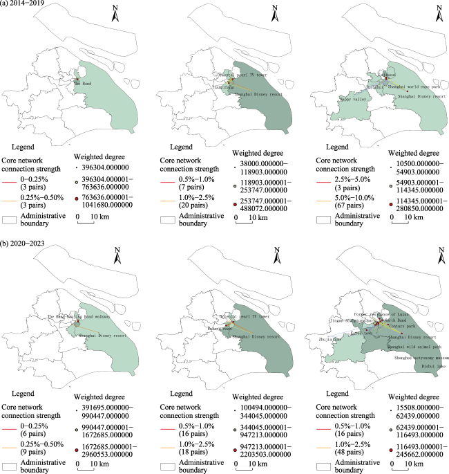
Figure 3 Spatial evolution of network linkages in the two phases |
| [1] |
|
| [2] |
|
| [3] |
|
| [4] |
|
| [5] |
|
| [6] |
|
| [7] |
|
| [8] |
|
| [9] |
|
| [10] |
|
| [11] |
|
| [12] |
|
| [13] |
|
| [14] |
|
| [15] |
|
| [16] |
|
| [17] |
|
| [18] |
|
| [19] |
|
| [20] |
|
| [21] |
|
| [22] |
|
| [23] |
|
| [24] |
|
| [25] |
|
| [26] |
|
| [27] |
|
| [28] |
|
| [29] |
|
| [30] |
|
| [31] |
|
| [32] |
|
| [33] |
|
| [34] |
|
| [35] |
|
| [36] |
|
| [37] |
|
| [38] |
|
| [39] |
|
| [40] |
|
| [41] |
|
| [42] |
|
| [43] |
|
| [44] |
|
| [45] |
|
| [46] |
|
| [47] |
|
| [48] |
|
| [49] |
|
| [50] |
|
| [51] |
|
| [52] |
|
| [53] |
|
| [54] |
|
| [55] |
|
| [56] |
|
| [57] |
|
| [58] |
|
| [59] |
|
| [60] |
|
| [61] |
|
/
| 〈 |
|
〉 |