Rural Revitalization and Agricultural Development

The Spatiotemporal Characteristics and Driving Factors of Agricultural Carbon Emissions in the Yellow River Basin

  • NIE Lei , 1 ,
  • BAO Xueli 1 ,
  • SUN Quan , 2, *
Expand
  • 1. Research Institute of Resource-based Economic Transformation and Development, Shanxi University of Finance and Economics, Taiyuan 030006, China
  • 2. Intelligent Management Accounting Institute, Shanxi University of Finance and Economics, Taiyuan 030006, China
* SUN Quan, E-mail:

NIE Lei, E-mail:

Received date: 2024-03-20

  Accepted date: 2024-07-10

  Online published: 2025-03-28

Supported by

The Humanities and Social Science Project of Ministry of Education(22YJAZH124)

The Philosophy and Social Sciences Research of Higher Learning Institutions of Shanxi(2022J019)

The Basic Research Program Project of Shanxi(202203021212494)

Shanxi Scholarship Council of China(2024-101)

The General Research Project on Socioeconomic Statistics of Shanxi(2024Z023)

Abstract

As the severity of climate change escalates, agriculture, being one of the primary contributors to global carbon emissions, has progressively come under scrutiny. Thus, fostering a low-carbon agriculture system is paramount in achieving the ambitious “dual carbon” goals of reaching peak carbon and attaining carbon neutrality. This study engages urban panel data from the Yellow River Basin spanning 2001-2020 to compute the agricultural carbon emissions therein. The research harnesses a spatial Durbin model to probe the influencing mechanisms and spatial effects while examining the implications of agricultural mechanization on such emissions. The findings reveal: (1) From a spatiotemporal perspective, total agricultural carbon emissions within the Yellow River Basin exhibited an oscillating “M”-shaped pattern. Upon analyzing spatial patterns, the carbon emissions were highest downstream, moderate midstream, and least upstream, signifying pronounced regional disparities. (2) Concerning the causal elements, agricultural mechanization, from a direct effects standpoint, tends to somewhat diminish local agricultural carbon emissions. Regarding spillover effects, agricultural mechanization similarly represses carbon emissions in adjacent locales. (3) Heterogeneity analysis suggests that in the midstream cities, agricultural mechanization results in a significant decrease in agricultural carbon emissions. Contrarily, upstream and downstream cities witness a stimulating effect. At present, with China’s agricultural economy navigating intense environmental pressure, these insights lend invaluable support to practices aimed at curbing agricultural carbon emissions. By shedding light on the interaction between agricultural mechanization and carbon emissions, they offer a novel perspective and empirical data. In turn, these can contribute to formulating policies that seek to reignite rural areas while concurrently striving to meet the strategic objectives of peak carbon and carbon neutrality.

Cite this article

NIE Lei , BAO Xueli , SUN Quan . The Spatiotemporal Characteristics and Driving Factors of Agricultural Carbon Emissions in the Yellow River Basin[J]. Journal of Resources and Ecology, 2025 , 16(2) : 457 -471 . DOI: 10.5814/j.issn.1674-764x.2025.02.015

1 Introduction

As China’s strategy for rural revitalization deepens, the sustainable growth of agriculture has taken center stage, concurrently spotlighting the issue of agricultural carbon emissions. A study by the Intergovernmental Panel on Climate Change (IPCC) informs that agriculture comprises 40% of CH4, 70% of N2O, and 20% of CO2 of the greenhouse gases emanating from human activities (Zhang et al., 2019). Moreover, data from the Food and Agriculture Organization (FAO) of the United Nations reveal that China, a significant agricultural producer, clocked in at approximately 90.3092 million t of agricultural carbon emissions in 2020—standing as the global leader in this metric . Consequently, curtailing agricultural carbon emissions in China is an escalating necessity (Choudhary et al., 2018; Wiśniewski and Kistowski, 2018; Chen et al., 2022).
The Yellow River Basin—a significant ecological and agricultural production base in China—stands as a representative region impacted by global warming. The pronounced economic disparities coupled with aggravating challenges related to ecology and water resources further complicate the situation (Qing et al., 2023). Thus, highlighting the critical need to unearth the spatiotemporal pattern of agricultural carbon emissions in the Yellow River Basin, elucidate its key determinants, and understand its implications in the context of national strategies for ecological protection and high-quality development under the “dual carbon” goals of achieving peak carbon and carbon neutrality.
Presently, the academic fold has invested considerably in researching the calculation, influencing factors, region- specific differences, and spatiotemporal distribution aspects of agricultural carbon emissions. Initial explorations were primarily centered on singular perspectives such as agricultural land use activities (Houghton et al., 2012), livestock breeding (Xue et al., 2019; Shi et al., 2022), and agricultural material inputs (West and Marland, 2002). However, with the progression of research, a comprehensive measurement of agricultural carbon emissions emerged, encompassing the carbon footprint of the Qinghai-Tibet Plateau from a generalized agricultural emissions viewpoint (including both planting and breeding) (Tian et al., 2021), and appraising the agricultural carbon emissions across 31 provinces and cities of China (excluding Taiwan, Hong Kong, and Macao due to missing data in these regions) based on 23 major emission sources including agricultural inputs, paddy fields, soil, livestock (Tian et al., 2014). This makes the accounting of agricultural carbon emissions more thorough.
In terms of influencing factors and research methodologies, several studies predominantly employ the Kaya identity (Li et al., 2014; Okorie and Lin, 2022), Logarithmic Mean Divisia Index (LMDI) (Zhao et al., 2018; Guo et al., 2021), STIRPAT model (Yang et al., 2021; Aziz and Chowdhury, 2023), and the Environmental Kuznets Curve (EKC) to investigate the components influencing agricultural carbon emissions (Balsalobre-Lorente et al., 2019; Ridzuan et al., 2020). These aspects encompass agricultural production facilities (Bai et al., 2023), agricultural policies (Chen et al., 2017; Du et al., 2023), economic progression (Dong et al., 2018), environmental regulation alongside fiscal decentralization (Ahmed et al., 2023; Xiong et al., 2023), industrial upgrading (Wei et al., 2023a), and energy consumption (Xu et al., 2021; Zhang and Li, 2022).
In line with this, scholars have examined the regional differences and the spatiotemporal dynamics of agricultural carbon emissions. The outcomes depict an ascending trend in China’s overall agricultural carbon emissions while the intensity of these emissions is on the decline (Huang et al., 2019). Furthermore, China’s planting sector showcases considerable disparities in agricultural carbon emission intensity (CEI) and per capita agricultural carbon emissions (CEPC). Regions with high CEI are predominantly agriculture-centric, whereas regions with high CEPC primarily lie in the northeastern and central areas renowned for their extensive planting operations (Cui et al., 2021). Thus, the regional differences in China’s agricultural carbon emissions are markedly significant (Cai et al., 2018; Pang et al., 2020).
In summary, existing research on agricultural carbon emissions is fairly comprehensive and systematic, encompassing aspects including the development of calculation indicators, analysis of spatiotemporal features, and exploration of influencing mechanisms—it lays a solid foundation for subsequent investigations. Nevertheless, existing studies exhibit limitations. There’s a lack of uniformity in the methodologies for calculating agricultural carbon emissions, some emission sources are overlooked, and the research perspectives are overwhelmingly concentrated at a macro level. Additionally, scant literature discusses the correlation between agricultural mechanization and agricultural carbon emissions, and there’s a dearth of analysis regarding the impact mechanism of agricultural mechanization on agricultural carbon emissions from the vantage point of spatial spillover.
Thus, this paper offers the following marginal contributions: Firstly, it rebuilds the indicator system—from the perspective of both planting and breeding carbon sources and agricultural carbon sinks—to systematically compute the agricultural carbon emissions of 99 prefecture-level cities in the Yellow River Basin. This expands the agricultural carbon emissions assessment system and broadens the research scale. Secondly, this paper investigates the relationship between agricultural mechanization and agricultural carbon emissions from a spatial standpoint, supplementing the interrelation between the two. Thirdly, taking into account spatial variations, it sheds light on the regional disparities in agricultural carbon emissions in the Yellow River Basin, explores the evolution pattern of these regional differences, and delves into the mechanisms behind spatial differentiation. Our aim is to formulate efficient agricultural carbon emission reduction mechanisms at the levels of the entire basin and basin subregions. This will ultimately offer insights for regional sustainable development decision- making.
The rest of this paper is arranged as follows: Section 2 pertains to the research design and explanation, Section 3 unveils the results, Section 4 takes on the discussion of the results, and Section 5 zeroes in on the conclusions of this research.

2 Material and methods

2.1 Model setting

2.1.1 Construction of the weight matrix

Selecting the appropriate spatial weight matrix is fundamental for performing spatial autocorrelation tests and spatial econometric model regression. Since certain cities in the Yellow River Basin are not adjacent, this study opts for the utilization of the economic geography nested matrix and geographic distance weight matrix for analysis (Gong et al., 2022).
Geographical distance weight matrix (W1):
$W1=\left\{ \begin{matrix} \frac{1}{{{d}_{ij}}^{2}},\ \ i\ne j \\ \ \ 0,\ \ i=j \\\end{matrix} \right.$.
In the formula, dij represents the distance between region i and j.
The economic distance weight matrix (W2):
$W2=\left\{ \begin{matrix} \frac{1}{\left| \overline{{{y}_{i}}}-\overline{{{y}_{j}}} \right|},\ \ i\ne j \\ 0 i=j \\\end{matrix} \right.$
In the formula, $\overline{{{y}_{i}}}$, $\overline{{{y}_{j}}}$ represent the per capita GDP of region i and j.
Economic geographical nested matrix (W3):
W3=$\varphi W1$+(1$\varphi $)W2
In the formula, $\varphi $ ranging from 0 to 1, represents the proportional weight of the geographical distance matrix, and for simplicity of analysis, $\varphi $ is taken as 0.5 (Hou et al., 2023).

2.1.2 Spatial autocorrelation analysis

The Global Moran’s Index is utilized in this study for spatial autocorrelation to test the spatial autocorrelation of different indicators. The objective is to look into the degree of spatial association of agricultural carbon emissions between cities and their neighboring cities. The formula for the Global Moran’s I Index is as follows:
$I=\frac{n\sum\limits_{i=1}^{n}{\sum\limits_{j=1}^{n}{{{w}_{ij}}}}\left( {{r}_{i}}-\bar{r} \right)\left( {{r}_{j}}-\bar{r} \right)}{\sum\limits_{i=1}^{n}{\sum\limits_{j=1}^{n}{{{w}_{ij}}{{\left( {{r}_{i}}-\bar{r} \right)}^{2}}}}}$
In this formula, n represents the number of spatial locations, ${{w}_{ij}}$ is the spatial weight matrix, representing the spatial relationship between units i and j; ${{r}_{i}}$ and ${{r}_{j}}$ represent the agricultural carbon emissions of each city, and $\bar{r}$ is the mean value.
The Global Moran’s I index ranges from [-1, 1]. When I=0, it indicates that agricultural carbon emissions are spatially unrelated and randomly distributed in space. When I<0, it signifies the presence of negative spatial correlation, showing a dispersed pattern. When I>0, it represents positive spatial correlation, indicating a clustered characteristic.

2.1.3 Spatial econometric model

This study empirically tests the spatial spillover effects of agricultural mechanization on agricultural carbon emissions using the Spatial Econometric Model. The formula is as follows:
$\begin{align} & \ln c{{e}_{it}}={{\alpha }_{0}}+\rho W\text{ln}c{{e}_{it}}+{{\beta }_{1}}Wl{{m}_{it}}+{{\gamma }_{1}}l{{m}_{it}}+ \\ & \ \ \ \ \ \ \ \ \ \ \ {{\gamma }_{2}}{{X}_{it}}+{{\beta }_{2}}W{{X}_{it}}+{{\mu }_{i}}+{{\eta }_{t}}+{{\varepsilon }_{it}} \\ \end{align}$
In this formula,$\ln c{{e}_{it}}$ represents agricultural carbon emissions, $l{{m}_{it}}$ represents agricultural mechanization,$\rho $ is the spatial correlation coefficient, W represents the spatial weight matrix,${{X}_{it}}$ represents control variables,subscript i indicates the i city, and t indicates the t year. ${{\alpha }_{0}}$ is a constant term,${{\beta }_{1}}$,${{\beta }_{2}}$ ${{\gamma }_{1}}$, ${{\gamma }_{2}}$ are coefficients to be estimated, ${{\mu }_{i}}$ and ${{\eta }_{t}}$ respectively represent individual and time effects,${{\varepsilon }_{it}}$ it is the random disturbance term.

2.1.4 Selection of models for testing spatial effects

After opting for spatial econometric models for empirical research, the selection of the appropriate model is determined through LM, Wald, and LR tests (Table 1). The LM test results show significance at the 1% level for both the Spatial Error Model (SEM) and the Spatial Autoregressive Model (SAR), suggesting that the Spatial Durbin Model (SDM) outperforms both. Subsequent LR and Wald tests also show significant results, indicating that the SDM model does not degenerate into the SAR or SEM models. The Hausman test is passed, suggesting that choosing a fixed-effects model is preferable to a random-effects model. In conclusion, the fixed-effects SDM model is chosen to explore the impact of agricultural mechanization on agricultural carbon emissions, with the regression results mainly analyzed using an economic geography nested matrix.
Table 1 Results of spatial panel model selection
Variables Statistics P-value Variables Statistics P-value
LM-Lag 697.033 <0.001 LR-SDM-SEM 206.47 <0.001
Robust LM-Lag 98.819 <0.001 LR-SDM-SAR 195.54 <0.001
LM-Error 694.283 <0.001 Wald-SDM-SEM 41.95 <0.001
Robust LM-Error 95.068 <0.001 Wald-SDM-SAR 31.65 <0.001
Hausman 122.39 <0.001

2.2 Variable measurement and explanation

2.2.1 Agricultural carbon emissions

Agricultural carbon emissions (ce). This study integrates different carbon sources in agricultural carbon emissions to establish a measurement index system. It includes five dimensions in both planting and breeding industries: agricultural product input, agricultural energy utilization, crop planting and growth, livestock enteric fermentation, and livestock manure management. The details are shown in Table 2.
Table 2 Agricultural carbon emission measurement index system
Dimensions Specific content
Agricultural inputs Fertilizers, pesticides, agricultural film
Agricultural energy use Electricity, diesel
Crop planting and growth Tillage, sowing and irrigation of rice, wheat, corn, legumes, cotton, vegetables, and other dryland crops
Livestock enteric
fermentation and livestock
manure management
Cows, pigs, sheep, horses, mules, donkeys, rabbits, poultry, camels

Note: The Yellow River Basin is known for planting winter wheat, hence the term “wheat” here specifically refers to winter wheat.

Using the carbon emissions factors provided by the Intergovernmental Panel on Climate Change (IPCC), we construct an agricultural carbon emissions measurement index system. This is done by calculating the product of the emissions volume for each carbon source and its corresponding emissions factor, yielding the volume of greenhouse gas emissions. Following this, the emissions are converted into carbon-equivalent emissions utilizing the Global Warming Potential (GWP) values for different gases. This process results in the total carbon emissions. The formula used to achieve this is as follows:
${{E}_{i}}={{T}_{i}}{{\delta }_{i}}$
$E=\mathop{\sum }^{}{{E}_{i}}{{\mu }_{i}}$
In the formula, ${{E}_{i}}$ represents the emission volume of agricultural greenhouse gases; ${{T}_{i}}$ is the volume of each carbon source; ${{\delta }_{i}}$ is the greenhouse gas coefficient caused by each carbon source; E is the total carbon emission volume; and ${{\mu }_{i}}$ is the Global Warming Potential value of
each greenhouse gas. According to the latest IPCC report, the Global Warming Potential values of methane and nitrous oxide are respectively 28-36 and 265-298 (with carbon dioxide’s value being 1), and this study uses their respective average values of 32 and 281.5. The original unit for carbon elements is multiplied by 44/12 to standardize it as carbon dioxide. The specific values of other coefficients are as detailed in Table 3 and Table 4.
Table 3 Agricultural carbon emission coefficient
Dimension Category Coefficient Unit
Agricultural product input Fertilizers 32838.67 t (CO2) Mt-1
Pesticides 180917.00 t (CO2) Mt-1
Agricultural film 189933.33 t (CO2) Mt-1
Agricultural energy use Electricity 2.90 t (CO2) Wh-1
Diesel 21732.33 t (CO2) Mt-1
Crop planting and growth Tillage 1146.20 t (CO2) kha-1
Sowing Wheat 492.63 t (CO2) kha-1
Corn 712.20 t (CO2) kha-1
Cotton 135.23 t (CO2) kha-1
Rice Qinghai 2253.16 t (CO2) kha-1
Sichuan 5484.09 t (CO2) kha-1
Gansu 2253.16 t (CO2) kha-1
Ningxia 2419.56 t (CO2) kha-1
Inner Mongolia 2925.16 t (CO2) kha-1
Shaanxi 4070.76 t (CO2) kha-1
Shanxi 2057.96 t (CO2) kha-1
Henan 5779.56 t (CO2) kha-1
Shandong 6787.56 t (CO2) kha-1
Soybean 644.64 t (CO2) kha-1
Vegetables 1390.61 t (CO2) kha-1
Other dryland crops 267.43 t (CO2) kha-1
Irrigation 91.67 t (CO2) kha-1
Table 4 Livestock carbon emission coefficient
Livestock Livestock enteric fermentation Livestock manure management
CH4 (kg) CH4 (kg) N2O (kg)
Cow 61.500 9.000 1.125
Donkey 10.000 0.900 1.390
Mule 10.000 0.900 1.390
Camel 46.000 1.920 1.390
Horse 18.000 1.640 1.390
Sheep 5.000 0.160 0.106
Pig 1.000 3.500 0.530
Rabbit 0.254 0.080 0.020
Poultry 0.000 0.020 0.020

Note: The above data is from Guidelines for compiling provincial greenhouse gas inventories; Oak Ridge National Laboratory in the United States (RNL); China Agricultural University (CAU); Institute of Agricultural Resources and Environmental Science, Nanjing Agricultural University (IREEA); Intergovernmental Panel on Climate Change (IPCC).
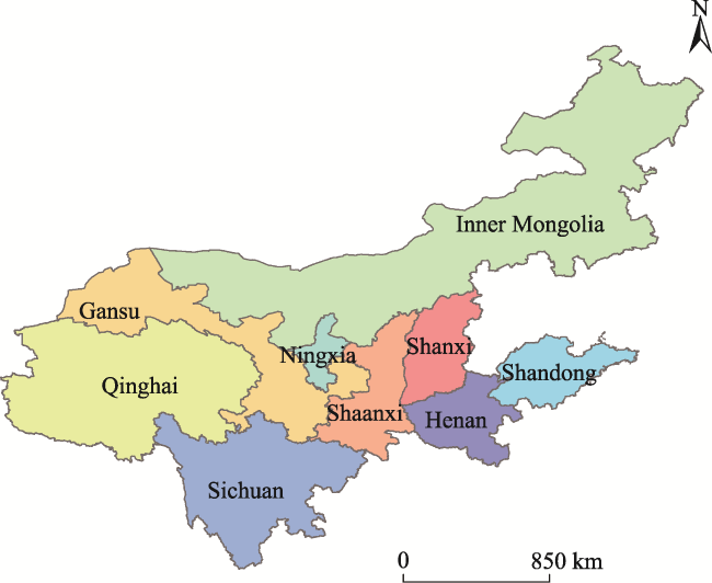
2.2.2 Core explanatory variable

Agricultural mechanization (lm). This study uses the total power of agricultural machinery relative to the total sown area of crops to measure the level of agricultural mechanization (Yang et al., 2022a).

2.2.3 Control variables

To eliminate the influence of other factors on the measurement results, this paper, referencing existing studies (Hu et al., 2022; Li et al., 2023; Wei et al., 2023b), incorporates the following control variables into the analysis for more comprehensive results. 1) Government support (gov): This variable is calculated as the ratio of forestry, agriculture, and water conservancy expenditures to the total output value of agriculture, forestry, animal husbandry, and fishery. 2) Urban-rural coordination (urban): The ratio of per capita living expenses of rural residents to urban residents is used as the standard of measurement. 3) Economic development level (pegdp): Represented by the actual per capita gross domestic product. 4) Rural industrial structure (industry): Calculated as the ratio of the total agricultural output value to the total output value of agriculture, forestry, animal husbandry, and fishery. 5) Urbanization rate (ur): Represented by the proportion of urban population to the total population.

2.3 Research area and data source

2.3.1 Research area

As shown in Figure 1, the Yellow River Basin holds significant ecological, economic, and cultural status in China. It does not only serve as a critical base for agricultural and energy production but also sports a unique geographical and climatic profile. With its boundaries stretching from 96°E to 119°E and 32°N to 42°N, the river flows from the west to the east, traversing nine provinces (and autonomous regions), which include Qinghai, Sichuan, Gansu, Ningxia, Inner Mongolia, Shanxi, Shaanxi, Henan, and Shandong, before making its way into the Bohai Sea.
The Yellow River Basin’s topographical complexity presents a fascinating landscape with a considerable elevation gradient. It features the west as the highest point with an average elevation surpassing 4000 m above sea level. The central region rests at an approximate altitude of 1000 to 2000 m, while the east comprises primarily of the Yellow River alluvial plain.
The climate mirrors the geographic diversity, featuring variations that notably influence the local agriculture— predominantly dryland farming. Interestingly, carbon emissions from these dryland soils share a close connection with global warming . Besides, the region’s delicate natural environment is particularly susceptible to irreversible ecological degradation (Xiong et al., 2016).
All these factors underscore the urgent need and relevance for a precise analysis of the agricultural carbon emis-sions and their associated influencers in the Yellow River Basin. Doing so offers valuable insights for realizing low- carbon agricultural development and enforcing effective ecological safeguards—both of which contribute meaningfully towards a sustainable future.

2.3.2 Data sources

This study utilizes the panel data from 99 cities located in the nine provinces of the Yellow River Basin, comprising data spanning from 2001 to 2020. The principal sources of this city-based data include publications such as the “China City Statistical Yearbook” (2000-2021), the “China Rural Statistical Yearbook” (2000-2021), and information drawn from the EPS database, among others.
Any gaps present in the data were addressed through the use of linear interpolation methods. Moreover, all price- related indicators were adjusted to align with the constant prices of the year 2001 to maintain the uniformity of data.
For a detailed descriptive statistical analysis of the variables, please refer to Table 5.
Table 5 Descriptive statistics of variables
Variable name Unit Observations Mean Std.dev Min Max
Agricultural carbon emissions (lnce) t 1980 14.815 1.139 9.250 17.168
Agricultural mechanization (lm) 104 kW kha-1 1980 0.691 0.656 0.107 20.815
Government support (gov) - 1980 0.171 0.151 0.025 0.955
Urban-rural coordination (urban) - 1980 0.412 0.116 0.190 0.794
Rural industrial structure (industry) - 1980 0.571 0.121 0.063 0.880
Economic development level (lnpegdp) yuan 1980 9.700 0.917 6.354 12.196
Urbanization rate (ur) - 1980 0.451 0.174 0.119 0.941

3 Results

3.1 Temporal and spatial evolution of agricultural carbon emission

3.1.1 Agricultural carbon emission temporal change

Figure 2 shows the trend of total agricultural carbon emissions in the Yellow River Basin from 2001 to 2020. Overall, the total carbon emissions from agriculture in the Yellow River Basin present an “M” shape, which can roughly be seen as four different stages: ‘fluctuating rise-fluctuating fall-slow rise-continuous fall.’ This indicates that agriculture is gradually moving towards low-carbon development. Specifically, from 2001 to 2004, agricultural carbon emissions showed an upward trend, followed by a significant decline after 2005. This may be due to China’s implementation of agricultural tax reduction and exemption policies from 2003, which, along with the development of agricultural cooperatives, promoted the scale of agricultural production, leading to an accelerated decline in agricultural carbon emissions from 2005 to 2007 (Cheng et al., 2023). After 2007, agricultural carbon emissions showed a slow upward trend. The reason might be that with the development of the social economy and the advancement of agricultural technology (Guo and Zhang, 2023), agricultural production efficiency was improved (Yin et al., 2017), which suppressed agricultural carbon emissions, but external economies had not yet formed. In 2015, a plan for zero growth in fertilizers and pesticides was introduced , and the ‘National Agricultural Modernization Plan (2016-2020)’ in 2016 explicitly proposed to fully implement the five development concepts, raise awareness of environmental protection, actively develop efficient green agriculture, and achieve agricultural modernization . Farmers began to shift from traditional agricultural production methods to green, low-carbon methods, engaging in low-carbon production or adopting low-carbon agricultural technologies, followed by a further decline in agricultural carbon emissions (Hu et al., 2022). Secondly, from the perspective of the regions shown in the figure, the carbon emissions from agriculture in the downstream area are far higher than those in the middle and upper reaches.
Figure 2 Total agricultural carbon emissions in the Yellow River Basin from 2001 to 2020

3.1.2 Spatial distribution of agricultural carbon emission levels

Figure 3 shows the spatial distribution of total agricultural carbon emissions in 2001, 2007, 2013, and 2020. Overall, the agricultural carbon emissions in the Yellow River Basin exhibit a pattern of “highest in the downstream, followed by the midstream, and lowest in the upstream,” with significant regional differences. From a spatial perspective: 1) The upstream area of the Yellow River Basin has lower agricultural carbon emissions. This may be due to the fact that the upstream area includes provinces such as Qinghai, Gansu, and Ningxia, which have harsh natural conditions and terrain consisting mostly of plateaus, deserts, and grasslands, unfavorable for large-scale agricultural production (Zhang et al., 2018). Additionally, the agricultural structure in these areas is predominantly livestock-based (Tian et al., 2021), which has lower carbon emissions compared to crop farming. 2) The midstream area of the Yellow River Basin includes Shanxi and Shaanxi provinces. Their agricultural carbon emissions are also relatively low. This may be due to these areas still relying on traditional agriculture with limited crop diversity. The development of livestock farming is relatively restricted, thus leading to lower carbon emissions. Shaanxi Province, in particular, exhibits a reverse “N” trend in agricultural carbon emissions. 3) The downstream area of the Yellow River Basin includes Henan and Shandong, two major grain-producing areas. Higher grain production means more agricultural carbon emissions. Additionally, the downstream area of the Yellow River Basin consists of more economically developed regions. The shift towards modern agriculture, along with extensive use of pesticides, fertilizers, and energy, also increases agricultural carbon emissions (Klasen et al., 2016). Currently, the downstream area of the Yellow River Basin remains a high agricultural carbon emission region.
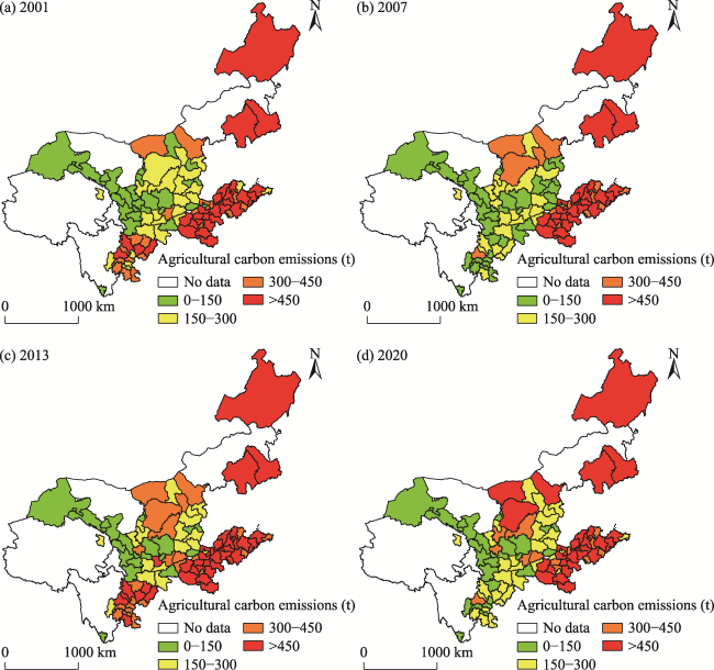
Figure 3 Spatial distribution of agricultural carbon emissions in the Yellow River Basin in 2001, 2007, 2013, and 2020
In summary, although the agricultural carbon emissions in the Yellow River Basin have shown a declining and fluctuating trend during the study period, there are still individual cities where agricultural carbon emissions have increased, with clear regional differences. Therefore, developing low- carbon agriculture will be a major measure for future agricultural carbon emission reduction in the Yellow River Basin (Chen et al., 2019).

3.2 Analysis of influencing factors

3.2.1 Global spatial autocorrelation test

The global Moran’s Index calculated according to the formula, as shown in Table 6, indicates that the Moran’s Index from 2001 to 2020 passed the significance test. This suggests that there is a certain degree of spatial dependency and spatial spillover effect in the agricultural carbon emissions in the Yellow River Basin. Moran’s I ranges from 0.149 to 0.208, showing little fluctuation, which indicates a stable spatial clustering effect in the agricultural carbon emissions of the Yellow River Basin. Furthermore, as can be seen from Table 6, the spatial correlation of agricultural carbon emissions has gradually weakened since 2008. This weakening may be due to the recent adjustments in industrial structure, with a significant increase in the proportions of the secondary and tertiary industries (Su et al., 2023). Additionally, the transformation in agricultural operation models is another factor. Modern agricultural operation models place more emphasis on sustainable development. Lastly, the government’s support for agriculture has been continuously increasing, with the introduction of a series of policies and measures encouraging farmers to adopt low-carbon and environmentally friendly production methods, such as promoting energy-saving and emission-reduction technologies (Yang et al., 2022b).
Table 6 Global Moran’s index
Year Moran’s I Z-statistics P-value Year Moran’s I Z-statistics P-value
2001 0.197 14.473 <0.001 2011 0.183 13.507 <0.001
2002 0.198 14.505 <0.001 2012 0.181 13.344 <0.001
2003 0.197 14.433 <0.001 2013 0.179 13.182 <0.001
2004 0.198 14.535 <0.001 2014 0.176 12.963 <0.001
2005 0.193 14.117 <0.001 2015 0.167 12.398 <0.001
2006 0.197 14.352 <0.001 2016 0.163 12.104 <0.001
2007 0.202 14.707 <0.001 2017 0.149 11.232 <0.001
2008 0.208 15.161 <0.001 2018 0.163 12.123 <0.001
2009 0.206 15.059 <0.001 2019 0.163 12.097 <0.001
2010 0.190 13.982 <0.001 2020 0.152 11.357 <0.001

3.2.2 Local spatial autocorrelation test

The Local Moran’s I scatter plot can be used to reveal the local evolutionary characteristics and differences in agricultural carbon emissions in the Yellow River Basin. Within this study, Moran’s scatter plots are created for the years 2001, 2007, 2013, and 2020, as shown in Figure 4. The Moran scatter plot categorizes cities into four quadrants based on their agricultural carbon emissions and their neighbors’ emissions: “High-High,” “Low-High,” “Low-Low,” and “High-Low”. These represent spatial relationships among cities. The “High-High” and “Low-Low” clusters indicate cities with similar high or low emissions surrounded by cities with the same trend, respectively. Conversely, “Low- High” and “High-Low” clusters show cities with emissions contrasting their neighbors’. Placement within the first and third quadrants signifies a high positive spatial correlation, indicating spatial uniformity, whereas placement within the second and fourth quadrants indicates a negative spatial correlation, signifying spatial heterogeneity. Across the selected years of 2001, 2007, 2013, and 2020, the distribution pattern of agricultural carbon emissions appears generally consistent. Most cities tend to fall into the first and third quadrants, thus forming either a “High-High” or “Low- Low” clustering trend, which suggests a positive spatial autocorrelation. Consequently, it can be deduced that there exists a stable spatial clustering effect in agricultural carbon emissions among the majority of cities within the Yellow River Basin.
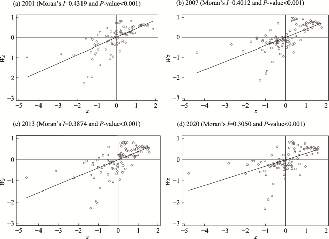
Figure 4 Moran’s scatter plots of agricultural carbon emissions in the Yellow River Basin for the years 2001, 2007, 2013, and 2020

3.2.3 Impact of agricultural mechanization on regional agricultural carbon emissions

The regression results of the spatial Durbin model are shown in Table 7. Table 7 presents the econometric results using an economic geographic distance-nested matrix. The results indicate that the direct effect of agricultural mechanization on agricultural carbon emissions is significantly negative at the 1% statistical level. Agricultural mechanization significantly reduces local agricultural carbon emissions, exhibiting a clear direct carbon reduction effect. The spatial spillover effect of agricultural mechanization on agricultural carbon emissions is also significantly negative at the 1% statistical level. A one-unit increase in the level of agricultural mechanization leads to a 7.566 unit decrease in agricultural carbon emissions in neighboring regions, demonstrating a significant spatial carbon reduction effect. The analysis suggests that considering the spatial spillover effect of agricultural mechanization, its carbon reduction impact will be even greater.
Table 7 Spatial econometric regression results
Variable Direct effect Indirect effect Total effect
lm -0.080*** -7.566*** -7.646***
(-3.62) (-3.77) (-3.77)
gov -0.280*** -22.260** -22.540**
(-2.77) (-2.26) (-2.26)
urban -0.585*** -58.083*** -58.669***
(-3.83) (-4.24) (-4.23)
industry -0.327*** -9.664 -9.990
(-2.26) (0.93) (-0.95)
lnpegdp 0.206*** 21.479*** 21.686***
(2.11) (2.98) (2.89)
ur -0.337*** -30.827*** -31.165***
(-2.78) (-3.11) (-3.11)
R2 0.003 0.003 0.003
Observations 1980 1980 1980

Note: ***P<0.01, **P<0.05, the t-value is enclosed in parentheses.

3.2.4 Results of the control variables measurement

From Table 7, it can be seen that among the control variables, policy support has a significant direct effect on agricultural carbon emissions at the 1% statistical level, and its spatial spillover effect and total effect on agricultural carbon emissions are significant at the 5% statistical level. Urban-rural coordination has a significantly negative direct effect, spatial spillover effect, and total effect on agricultural carbon emissions at the 1% statistical level. The rural industrial structure has a significantly negative direct effect on agricultural carbon emissions at the 1% statistical level, but its spatial spillover effect and total effect on agricultural carbon emissions are not significant. The level of economic development has a significantly positive direct effect, spatial spillover effect, and total effect on agricultural carbon emissions at the 1% statistical level. The level of urbanization has a significantly negative direct effect, spatial spillover effect, and total effect on agricultural carbon emissions at the 1% statistical level.

3.3 Robustness test

To ensure more rigorous validation of the benchmark regression outcomes, we undertook the following robustness tests: 1) Substitution of the spatial weight matrix: We replaced the current spatial weight matrix with a geographical distance weight matrix for the test. 2) Alteration of the explanatory variables’ measurement indicators: Utilizing the entropy weight method, we gauged the level of agricultural mechanization, the degree of agricultural electrification, and the level of effective irrigation. The results derived were then employed as surrogate variables for agricultural mechanization. 3) Bilateral truncation of variables: This was done to mitigate the influence of outliers in the model which could potentially affect the accuracy of the estimation results. We trimmed the variables bilaterally at the 1% quantile and proceeded with the regression. The findings from these tests are presented in Table 8.
Table 8 Robustness check results
Spatial effects Variable (1) (2) (3)
Direct effect lm -0.078*** -2.292*** -0.103**
(-3.19) (-3.29) (-2.49)
gov -0.346*** -0.245*** -0.230**
(-3.14) (-2.60) (-2.31)
urban -0.877*** -0.579*** -0.725***
(-4.08) (-3.86) (-4.50)
industry -0.088 -0.320** -0.276*
(-0.51) (-2.26) (-1.72)
lnpegdp 0.008 0.165* -0.025
(0.09) (1.77) (-0.30)
ur -0.777*** -0.298** -0.309**
(-4.12) (-2.53) (-2.53)
Spatial spillover effect lm -7.661*** -216.920*** -12.982***
(-3.38) (-3.46) (-3.55)
gov -21.863** -18.007** -17.871*
(-1.97) (-1.97) (-1.83)
urban -83.154*** -57.580*** -62.510***
(-4.07) (-4.30) (-4.29)
industry 19.131 -9.977 2.968
(1.41) (-1.01) (0.25)
lnpegdp 0.486 19.167*** 13.365**
(0.06) (2.77) (2.06)
ur -70.562*** -28.219*** -24.945**
(-4.04) (-3.00) (-2.50)
Total effect lm -7.738*** -219.211*** -13.085***
(-3.38) (-3.46) (-3.55)
gov -22.209** -18.252** -18.101*
(-1.99) (-1.98) (-1.84)
urban -84.031 *** -58.159*** -63.235***
(-4.07) (-4.30) (-4.29)
industry 19.044 -10.297 2.692
(1.39) (-1.04) (0.22)
lnpegdp 0.494 19.332*** 13.340**
(0.06) (2.77) (2.03)
ur -71.339*** -28.517*** -25.254**
(-4.04) (-3.00) (-2.51)
R2 0.000 0.003 0.003
Observations 1980 1980 1980

Note: ***P<0.01, **P<0.05, * P<0.1, the t-value is enclosed in parentheses.

Columns (1) to (3) in Table 8 systematically display the outcomes of the previously described three robustness tests. A point of significance is that the spatial spillover effect of agricultural mechanization on agricultural carbon emissions has consistently shown a significant negative correlation, regardless of the method employed. This reaffirms the dependability and robustness of our baseline regression analyses, thereby adding weight to our findings. It indeed suggests that agricultural mechanization plays a key role in reducing agricultural carbon emissions not only locally, but it also has a positive spillover effect on neighboring areas.

3.4 Heterogeneity analysis

This study further examines the regional heterogeneity of the impact of agricultural mechanization on agricultural carbon emissions in different areas. Based on the geographical location of the Yellow River Basin, it is divided into three regions: the upper, middle, and lower reaches. The regression results are shown in columns (1), (2), and (3) of Table 9, respectively. From a regional perspective, agricultural mechanization significantly inhibited agricultural carbon emissions in the middle reaches of the Yellow River at the 1% level. In contrast, agricultural mechanization has shown a significant positive impact on agricultural carbon emissions in the upper and lower reaches of the Yellow River, and their estimated coefficients have passed the 1% significance test. The spatial spillover effects of several factors on agricultural carbon emissions in different regions of the Yellow River Basin are significant, as follows:
Table 9 Heterogeneity analysis
Spatial effects Various (1) (2) (3)
Direct effect lm 0.118*** -0.025*** 0.111***
(3.01) (-2.65) (3.40)
gov -1.023*** 0.048 -0.458***
(-4.50) (0.65) (-3.04)
urban -0.422** 0.009 0.085
(-2.07) (0.13) (0.83)
industry -0.238 -0.683*** -0.929***
(-0.94) (-4.49) (-7.10)
lnpegdp -0.519** 0.400*** 0.380***
(-2.57) (5.01) (3.50)
ur -0.401 -0.525*** -0.019
(-1.06) (-4.38) (-0.34)
Spatial spillover effect lm 3.564*** -0.833*** 1.255***
(3.10) (-4.31) (3.81)
gov -29.197*** -4.740*** 0.352
(-3.56) (-3.07) (0.24)
urban -14.718*** 0.792 0.686
(-2.63) (0.86) (1.04)
industry -17.661** -3.073 0.924
(-2.56) (-1.40) (0.96)
lnpegdp -22.972*** 3.315*** 1.420
(-4.00) (3.31) (1.63)
ur -23.460** -8.223*** -0.154
(-2.03) (-3.83) (-0.27)
Total effect lm 3.682*** -0.858*** 1.366***
(3.11) (-4.29) (4.19)
gov -30.221*** -4.692*** -0.106
(-3.59) (-2.94) (-0.07)
urban -15.140*** 0.802 0.771
(-2.62) (0.84) (1.17)
industry -17.899** -3.756* -0.005
(-2.53) (-1.66) (-0.01)
lnpegdp -23.491*** 3.715*** 1.800**
(-3.99) (3.64) (2.04)
ur -23.861** -8.748*** -0.173
(-2.00) (-3.95) (-0.30)
R2 0.001 0.003 0.012
Observations 720 600 660

Note: ***P<0.01, **P<0.05, *P<0.1, the t-value is enclosed in parentheses.

In the upper reaches of the Yellow River Basin, policy support, urban-rural coordination, the level of economic development, the structure of the rural industry, and the rate of urbanization all have notable negative spatial spillover effects on agricultural carbon emissions. This indicates that these areas are effectively leveraging these factors to reduce carbon emissions in agriculture, which not only impacts their immediate vicinity but also neighboring regions.
Likewise, in the middle reaches of the Yellow River Basin, policy support, the level of economic development, and the rate of urbanization are seen to have significant negative spatial spillover effects on agricultural carbon emissions.
This suggests that improvements in these areas can contribute to a reduction in agricultural carbon emissions, affecting not only the local region but also adjacent areas.
By understanding the influence of these factors, policy makers can drive more effective strategies targeted toward reducing agricultural carbon emissions and mitigating the impact of climate change in this crucial watershed.
In conclusion, the development disparities within the Yellow River Basin influence how agricultural mechanization affects agricultural carbon emissions in this region. It’s clear that the impact of mechanization fluctuates depending on various elements unique to each area within the basin. The findings of our research provide a strong theoretical foundation for tailored development of low-carbon agriculture across the Yellow River Basin.

4 Discussion

4.1 Spatial-temporal pattern of agricultural carbon emissions

Our investigation revealed that, as a general trend, agricultural carbon emissions in the Yellow River Basin were decreasing throughout the duration of our study, notwithstanding a few fluctuations perceived in the mid-term analysis. However, some regions diverged from this general trend, showing an increase in their agricultural carbon emissions instead.
Spatial analysis presents a significant regional disparity in terms of these emissions across the Yellow River Basin, which echoes the findings of Chen et al. (2019) and Zhang et al. (2022). We believe these disparities can be attributed to the significant regional differences in climate conditions and resource endowments within the Basin, which consequently reflect on the varied conditions of agricultural production in each respective area. This variance in agricultural contexts is instrumental in generating the apparent regional disparity in agricultural carbon emissions, as indicated in Huang et al. (2019)’s study.

4.2 Factors influencing agricultural carbon missions

This study primarily focused on investigating the correlation between agricultural mechanization and agricultural carbon emissions. Our empirical findings recognize that agricultural mechanization substantially reduced local agricultural carbon emissions. Moreover, it also had a pronounced negative spatial spillover effect, implying a distinctly noticeable spatial carbon reduction effect. These insights collectively further affirm the findings reached by Guo and Zhang in 2023.
The key reasons driving this spatial spillover effect can be classified into two main strands.
Firstly, the incorporation of agricultural machinery enables operations across a broad range of regions, thus overcoming potential limitations such as inconsistent land ownership and fragmented landholdings (Hao et al., 2023). This leads to the enhancement of land-use efficiency (Kuang et al., 2020), enabling large-scale mechanized operations (Ren et al., 2019) and fostering agricultural specialization (Wang et al., 2022). As an immediate outcome, this reduces both the average cost and carbon emissions per production unit (Lu et al., 2018).
Secondly, the demonstration effect holds considerable weight. The influence of agricultural mechanization isn’t restricted to individual farmers or specific regions. Instead, it exhibits a spillover effect on the neighboring areas. Facilitating shared infrastructure across regions, agricultural mechanization promotes the enhancement of both agricultural production technology and the efficiency of agricultural inputs.
The demonstration effect spins a web of imitation and competition among surrounding areas, weaving a wider adoption region for agricultural mechanization through the transfer of technology know-how and experiences. Consequently, farmers nestled in neighboring areas can access machinery services and technical knowledge at reduced costs, eventually fostering carbon reduction in agricultural production in these areas too (Qayyum et al., 2023; Rong et al., 2023).
In light of these findings, it is beneficial for the government to provide conditions conducive to the broader implementation of agricultural mechanization. This could be achieved by leveraging methods like fiscal subsidies and tax incentives, which could accelerate the high-quality development of low-carbon agriculture.
Upon further consideration of other influential factors highlighted in Table 7, we see that government initiatives aimed at enhancing agricultural technology, incentivizing shifts in agricultural business models and providing green subsidies and rewards have been successful in reducing local agricultural carbon emissions (Solazzo et al., 2016; Xu and Lin, 2017).
Economic growth, on the other hand, contributed to an increase in agricultural carbon emissions, which aligns with the conclusions drawn by Wang et al. (2020) and Raihan et al. (2023). Han et al. (2022) posits that the coordinated development of urban and rural areas has resulted in a decrease in the proportion of coal used in rural life, in tandem with an increase in the consumption of clean energy in agricultural production, both factors leading to carbon reduction. Further, the level of urbanization, reflective of regional economic progress, has an interesting effect. As urbanization levels rise, the consumption of agricultural resources begins to decrease. Changes in urban lifestyles and resource utilization methods have, to an extent, reduced the carbon emissions related to agriculture (Zhang et al., 2017; Prastiyo et al., 2020).
Examining the heterogeneity presented in Table 9, it’s interesting to note that agricultural mechanization’s inhibitory effect on carbon emissions is significantly more pronounced in the middle cities of the Yellow River Basin, while it seems to promote carbon emissions in both the upstream and downstream regions.
The main reason for this disparity could be the focused policy support, accelerating the promotion and popularization of agricultural mechanization in the middle reaches of the Yellow River Basin. The implementation of agricultural mechanization aids in attaining an economy of scale, minimizes energy consumption and paves the way for precision fertilization and water conservation in irrigation-ultimately decreasing the usage of fertilizers and pesticides and further reducing carbon emissions (Su et al., 2022).
In the upstream regions, where natural conditions are harsh and the agricultural method is mainly livestock-based, agricultural mechanization isn’t beneficial. In the economically advanced downstream regions, substantial amounts of energy and fertilizers are expended in the drive towards agricultural modernization, with these areas leaning more towards the cultivation of economically beneficial crops. Consequently, the external effects of agricultural mechanization in these downstream areas are not yet evident.

4.3 Limitations and future research directions

While our study has strived to provide a robust quantitative examination of agricultural carbon emissions, there remain areas for further exploration and enhancement. The intricate distinctions across different regions and varieties of crops have introduced a set of complexities that have constrained us from achieving full precision in the conclusive measurement of effectiveness.
Looking ahead, provided technology and data availability permit, our plan is to construct a more comprehensive and detailed system for calculating agricultural carbon emissions. Extending our scope of inquiry to encompass key factors influencing agricultural carbon emissions—such as land-use practices, agricultural policies, and farmers’ behaviors could yield insightful revelations.
Additionally, an imperative aspect that warrants our attention is how to orchestrate a harmonious balance between economic gains and ecological benefits. Achieving this equilibrium is paramount to fostering sustainable agricultural development, and thus, is a worthwhile endeavor for further research and consideration.

5 Conclusions and policy suggestions

5.1 Conclusions

In this study, we carried out an analysis based on collected panel data from 99 cities in the Yellow River Basin spanning from 2001 to 2020. We systematically computed agricultural carbon emissions after introducing an index system and then evaluated the timeline characteristics and spatial distribution of these emissions. By using the Spatial Durbin Model, we gauged the impact of agricultural mechanization and various other influencing elements on agricultural carbon emissions, drawing the following conclusions:
Firstly, Throughout the period under study, the total agricultural carbon emissions in the Yellow River Basin followed an “M” shaped fluctuation trend. From 2001 to 2004, emissions were on an incline. This was followed by a dramatic drop from 2004 to 2007. After 2007, the emissions began to rise again, experiencing a slower decline after 2016. Spatial analysis indicates that the regions downstream of the Yellow River Basin have the highest emissions, followed by those midstream, with upstream areas having the least. The findings show clear regional differentiation.
Secondly, The Spatial Durbin Model facilitated an understanding of direct and spillover effects of agricultural mechanization on agricultural carbon emissions. As far as direct effects are concerned, agricultural mechanization suppresses local agricultural carbon emissions. From a spillover effect perspective, agricultural mechanization also reduces agricultural carbon emissions in surrounding areas. Furthermore, factors such as policy support, coordination between urban and rural areas, and urbanization have significantly contributed to reducing agricultural carbon emissions in the Yellow River Basin.
Lastly, when we examine regional heterogeneity, the influence of agricultural mechanization on agricultural carbon emissions is more apparent in midstream cities of the Yellow River Basin. Therefore, based on the results of our analysis, we propose differentiated measures for agricultural emission reduction, which hold significant potential for advancing the development of low-carbon agriculture.

5.2 Policy suggestions

To promote sustainable and low-carbon agricultural development, we propose the following steps:
(1) Fostering agricultural technology innovation and furthering the modernization of agricultural practices. Enhanced investment in research and development is essential to discover and promote low-carbon agricultural technologies tailored to the needs and circumstances of the Yellow River Basin. Practices such as water-saving irrigation and precision fertilization can vastly improve the efficiency of agricultural production, thereby reducing carbon emissions.
(2) Transforming and optimizing agricultural production methods and industry structures. Primarily, there is a need to refashion the current crop cultivation setup. In a bid to lower high-carbon agricultural practices, advancements should be made toward transitioning traditional agriculture in the Yellow River Basin to more modern, greener, organic, and ecologically friendly farming methods. Secondly, the development of circular agriculture, utilizing clean energy and minimizing agricultural pollution, should be given due consideration.
(3) Amplifying policy support and development guidance. Government authorities should strive to refine relevant policies on carbon emissions in agriculture and boost financial backing, perhaps through the formulation of policies providing subsidies to agricultural productions. Moreover, it is advisable for local governments to consider adopting differentiated strategies while framing policies for reducing agricultural carbon emissions, keeping in mind the regional disparities within the Yellow River Basin. Appreciable efforts should also be made to raise awareness among farmers about agricultural carbon emission issues, encouraging them to actively participate in initiatives geared towards emission reduction.
[1]
Ahmed N, Hamid Z, Rehman K U, et al. 2023. Environmental regulation, fiscal decentralization, and agricultural carbon intensity: A challenge to ecological sustainability policies in the United States. Sustainability, 15 (6): 5145. DOI: 10.3390/su15065145.

[2]
Aziz S, Chowdhury S A. 2023. Analysis of agricultural greenhouse gas emissions using the STIRPAT model: A case study of Bangladesh. Environment, Development and Sustainability, 25(5): 3945-3965.

[3]
Bai Z, Wang T, Xu J, et al. 2023. Can agricultural productive services inhibit carbon emissions? Evidence from China. Land, 12(7): 1313. DOI: 10.3390/land12071313.

[4]
Balsalobre-Lorente D, Driha O M, Bekun F V, et al. 2019. Do agricultural activities induce carbon emissions? The BRICS experience. Environmental Science and Pollution Research, 26(24): 25218-25234.

DOI

[5]
Cai B F, Wang X Q, Huang G H, et al. 2018. Spatiotemporal changes of China’s carbon emissions. Geophysical Research Letters, 45(16): 8536-8546.

[6]
Chen M P, Cui Y R, Jiang S, et al. 2022. Toward carbon neutrality before 2060: Trajectory and technical mitigation potential of non-CO2 greenhouse gas emissions from Chinese agriculture. Journal of Cleaner Production, 368: 133186. DOI: 10.1016/j.jclepro.2022.133186.

[7]
Chen Y H, Li M J, Su K, et al. 2019. Spatial-temporal characteristics of the driving factors of agricultural carbon emissions: Empirical evidence from Fujian, China. Energies, 12(16): 3102. DOI: 10.3390/en12163102.

[8]
Chen Y H, Wen X W, Wang B, et al. 2017. Agricultural pollution and regulation: How to subsidize agriculture? Journal of Cleaner Production, 164: 258-264.

[9]
Cheng Q Y, Li L Y, Liao Q, et al. 2023. Is scale production more advantageous than smallholders for Chinese rice production? Energy, 283: 128753. DOI: 10.1016/j.energy.2023.128753.

[10]
Choudhary P, Srivastava R K, De S. 2018. Integrating Greenhouse gases (GHG) assessment for low carbon economy path: Live case study of Indian national oil company. Journal of Cleaner Production, 198: 351-363.

[11]
Cui Y, Khan S U, Deng Y, et al. 2021. Regional difference decomposition and its spatiotemporal dynamic evolution of Chinese agricultural carbon emission: Considering carbon sink effect. Environmental Science and Pollution Research, 28(29): 38909-38928.

[12]
Dong K Y, Sun R J, Jiang H D, et al. 2018. CO2 emissions, economic growth, and the environmental Kuznets curve in China: What roles can nuclear energy and renewable energy play? Journal of Cleaner Production, 196: 51-63.

[13]
Du Y, Liu H, Huang H, et al. 2023. The carbon emission reduction effect of agricultural policy-Evidence from China. Journal of Cleaner Production, 406: 137005. DOI: 10.1016/j.jclepro.2023.137005.

[14]
Gong W, Fan Z, Wang C, et al. 2022. Spatial spillover effect of carbon emissions and its influencing factors in the Yellow River Basin. Sustainability, 14 (6): 3608. DOI: 10.3390/su14063608.

[15]
Guo H, Fan B, Pan C. 2021. Study on mechanisms underlying changes in agricultural carbon emissions: A case in Jilin Province, China, 1998-2018. International Journal of Environmental Research and Public Health, 18 (3): 919. DOI: 10.3390/ijerph18030919.

[16]
Guo Z, Zhang X. 2023. Carbon reduction effect of agricultural green production technology: A new evidence from China. Science of the Total Environment, 874: 162483. DOI: 10.1016/j.scitotenv.2023.162483.

[17]
Han J S, Yang Q, Zhang L. 2022. What are the priorities for improving the cleanliness of energy consumption in rural China? Urbanisation advancement or agriculture development? Energy for Sustainable Development, 70: 106-114.

[18]
Hao W, Hu X, Wang J, et al. 2023. The impact of farmland fragmentation in China on agricultural productivity. Journal of Cleaner Production, 425: 138962. DOI: 10.1016/j.jclepro.2023.138962.

[19]
Hou L C, Tian C S, Xiang R B, et al. 2023. Research on the impact mechanism and spatial spillover effect of digital economy on rural revitalization: An empirical study based on China’s provinces. Sustainability, 15(15): 11607. DOI: 10.3390/su151511607.

[20]
Houghton R A, House J I, Pongratz J, et al. 2012. Carbon emissions from land use and land-cover change. Biogeosciences, 9(12): 5125-5142.

[21]
Hu C, Fan J, Chen J. 2022. Spatial and temporal characteristics and drivers of agricultural carbon emissions in Jiangsu Province, China. International Journal of Environmental Research and Public Health, 19(19): 12463. DOI: 10.3390/ijerph191912463.

[22]
Huang X Q, Xu X C, Wang Q Q, et al. 2019. Assessment of agricultural carbon emissions and their spatiotemporal changes in China, 1997-2016. International Journal of Environmental Research and Public Health, 16(17): 3105. DOI: 10.3390/ijerph16173105.

[23]
Klasen S, Meyer K M, Dislich C, et al. 2016. Economic and ecological trade-offs of agricultural specialization at different spatial scales. Ecological Economics, 122: 111-120.

[24]
Kuang B, Lu X, Zhou M, et al. 2020. Provincial cultivated land use efficiency in China: Empirical analysis based on the SBM-DEA model with carbon emissions considered. Technological Forecasting and Social Change, 151: 119874. DOI: 10.1016/j.techfore.2019.119874.

[25]
Li J, Gao M, Luo E, et al. 2023. Does rural energy poverty alleviation really reduce agricultural carbon emissions? The case of China. Energy Economics, 119: 106576. DOI: 10.1016/j.eneco.2023.106576.

[26]
Li W, Ou Q X, Chen Y L. 2014. Decomposition of China’s CO2 emissions from agriculture utilizing an improved Kaya identity. Environmental Science and Pollution Research, 21(22): 13000-13006.

[27]
Lu H, Xie H L, He Y F, et al. 2018. Assessing the impacts of land fragmentation and plot size on yields and costs: A translog production model and cost function approach. Agricultural Systems, 161: 81-88.

[28]
Okorie D I, Lin B Q. 2022. Emissions in agricultural-based developing economies: A case of Nigeria. Journal of Cleaner Production, 337: 130570. DOI: 10.1016/j.jclepro.2022.130570.

[29]
Pang J X, Li H J, Lu C P, et al. 2020. Regional differences and dynamic evolution of carbon emission intensity of agriculture production in China. International Journal of Environmental Research and Public Health, 17(20): 7541. DOI: 10.3390/ijerph17207541.

[30]
Prastiyo S E, Irham, Hardyastuti S, et al. 2020. How agriculture, manufacture, and urbanization induced carbon emission? The case of Indonesia. Environmental Science and Pollution Research, 27(33): 42092-42103.

[31]
Qayyum M, Zhang Y, Wang M, et al. 2023. Advancements in technology and innovation for sustainable agriculture: Understanding and mitigating greenhouse gas emissions from agricultural soils. Journal of Environmental Management, 347: 119147. DOI: 10.1016/j.jenvman.2023.119147.

[32]
Qing Y, Zhao B J, Wen C H. 2023. The coupling and coordination of agricultural carbon emissions efficiency and economic growth in the Yellow River Basin, China. Sustainability, 15(2): 971. DOI: 10.3390/su15020971.

[33]
Raihan A, Ibrahim S, Muhtasim D A. 2023. Dynamic impacts of economic growth, energy use, tourism, and agricultural productivity on carbon dioxide emissions in Egypt. World Development Sustainability, 2: 100059. DOI: 10.1016/j.wds.2023.100059.

[34]
Ren C C, Liu S, van Grinsven H, et al. 2019. The impact of farm size on agricultural sustainability. Journal of Cleaner Production, 220: 357-367.

DOI

[35]
Ridzuan N H A M, Marwan N F, Khalid N, et al. 2020. Effects of agriculture, renewable energy, and economic growth on carbon dioxide emissions: Evidence of the environmental Kuznets curve. Resources, Conservation and Recycling, 160: 104879. DOI: 10.1016/j.resconrec.2020.104879.

[36]
Rong J, Hong J, Guo Q, et al. 2023. Path mechanism and spatial spillover effect of green technology innovation on agricultural CO2 emission intensity: A case study in Jiangsu Province, China. Ecological Indicators, 157: 111147. DOI: 10.1016/j.ecolind.2023.111147.

[37]
Shi R B, Irfan M, Liu G L, et al. 2022. Analysis of the impact of livestock structure on carbon emissions of animal husbandry: A sustainable way to improving public health and green environment. Frontiers in Public Health, 10: 835210. DOI: 10.3389/fpubh.2022.835210.

[38]
Solazzo R, Donati M, Tomasi L, et al. 2016. How effective is greening policy in reducing GHG emissions from agriculture? Evidence from Italy. Science of the Total Environment, 573: 1115-1124.

[39]
Su L J, Wang Y T, Yu F F. 2023. Analysis of regional differences and spatial spillover effects of agricultural carbon emissions in China. Heliyon, 9(6): e16752. DOI: 10.1016/j.heliyon.2023.e16752.

[40]
Su M, Heerink N, Oosterveer P, et al. 2022. Upscaling farming operations, agricultural mechanization and chemical pesticide usage: A macro-analysis of Jiangsu Province, China. Journal of Cleaner Production, 380: 135120. DOI: 10.1016/j.jclepro.2022.135120.

[41]
Tian Y, Jiang G, Zhou D, et al. 2021. Systematically addressing the heterogeneity in the response of ecosystem services to agricultural modernization, industrialization and urbanization in the Qinghai-Tibetan Plateau from 2000 to 2018. Journal of Cleaner Production, 285: 125323. DOI: 10.1016/j.jclepro.2020.125323.

[42]
Tian Y, Zhang J B, He Y Y. 2014. Research on spatial-temporal characteristics and driving factor of agricultural carbon emissions in China. Journal of Integrative Agriculture, 13(6): 1393-1403.

DOI

[43]
Wang L, Vo X V, Shahbaz M, et al. 2020. Globalization and carbon emissions: Is there any role of agriculture value-added, financial development, and natural resource rent in the aftermath of COP21? Journal of Environmental Management, 268: 110712. DOI: 10.1016/j.jenvman.2020.110712.

[44]
Wang R R, Zhang Y, Zou C M. 2022. How does agricultural specialization affect carbon emissions in China? Journal of Cleaner Production, 370: 133463. DOI: 10.1016/j.jclepro.2022.133463.

[45]
Wei S L, Yang Y S, Xu Y. 2023a. Regional development, agricultural industrial upgrading and carbon emissions: What is the role of fiscal expenditure?-Evidence from Northeast China. Economic Analysis and Policy, 80: 1858-1871.

[46]
Wei Z Q, Wei K K, Liu J C, et al. 2023b. The relationship between agricultural and animal husbandry economic development and carbon emissions in Henan Province, the analysis of factors affecting carbon emissions, and carbon emissions prediction. Marine Pollution Bulletin, 193: 115134. DOI: 10.1016/j.marpolbul.2023.115134.

[47]
West T O, Marland G. 2002. A synthesis of carbon sequestration, carbon emissions, and net carbon flux in agriculture: Comparing tillage practices in the United States. Agriculture, Ecosystems & Environment, 91(1-3): 217-232.

[48]
Wiśniewski P, Kistowski M. 2018. Assessment of greenhouse gas emissions from agricultural sources in order to plan for needs of low carbon economy at local level in Poland. Geografisk Tidsskrift-Danish Journal of Geography, 118(2): 123-136.

[49]
Xiong C H, Yang D G, Xia F Q, et al. 2016. Changes in agricultural carbon emissions and factors that influence agricultural carbon emissions based on different stages in Xinjiang, China. Scientific Reports, 6: 36912. DOI: 10.1038/srep36912.

PMID

[50]
Xiong H, Zhan J T, Xu Y J, et al. 2023. Challenges or drivers? Threshold effects of environmental regulation on China’s agricultural green productivity. Journal of Cleaner Production, 429: 139503. DOI: 10.1016/j.jclepro.2023.139503.

[51]
Xu B, Lin B Q. 2017. Factors affecting CO2 emissions in China’s agriculture sector: Evidence from geographically weighted regression model. Energy Policy, 104: 404-414.

[52]
Xu X C, Yang H M, Yang H R. 2021. The threshold effect of agricultural energy consumption on agricultural carbon emissions: A comparison between relative poverty regions and other regions. Environmental Science and Pollution Research, 28(39): 55592-55602.

[53]
Xue Y N, Luan W X, Wang H, et al. 2019. Environmental and economic benefits of carbon emission reduction in animal husbandry via the circular economy: Case study of pig farming in Liaoning, China. Journal of Cleaner Production, 238: 117968. DOI: 10.1016/j.jclepro.2019.117968.

[54]
Yang H, Wang X X, Bin P. 2022a. Agriculture carbon-emission reduction and changing factors behind agricultural eco-efficiency growth in China. Journal of Cleaner Production, 334: 130193. DOI: 10.1016/j.jclepro.2021.130193.

[55]
Yang Y Y, Tian Y, Peng X H, et al. 2022b. Research on environmental governance, local government competition, and agricultural carbon emissions under the goal of carbon peak. Agriculture, 12(10): 1703. DOI: 10.3390/agriculture12101703.

[56]
Yang X, Jia Z, Yang Z, et al. 2021. The effects of technological factors on carbon emissions from various sectors in China-A spatial perspective. Journal of Cleaner Production, 301: 126949. DOI: 10.1016/j.jclepro.2021.126949.

[57]
Yin W, Chai Q, Guo Y, et al. 2017. Reducing carbon emissions and enhancing crop productivity through strip intercropping with improved agricultural practices in an arid area. Journal of Cleaner Production, 166: 197-208.

[58]
Zhang C Y, Zhao L, Zhang H T, et al. 2022. Spatial-temporal characteristics of carbon emissions from land use change in Yellow River Delta region, China. Ecological Indicators, 136: 108623. DOI: 10.1016/j.ecolind.2022.108623.

[59]
Zhang H S, Li S P. 2022. Carbon emissions’ spatial-temporal heterogeneity and identification from rural energy consumption in China. Journal of Environmental Management, 304: 114286. DOI: 10.1016/j.jenvman.2021.114286.

[60]
Zhang L, Pang J X, Chen X P, et al. 2019. Carbon emissions, energy consumption and economic growth: Evidence from the agricultural sector of China’s main grain-producing areas. The Science of the Total Environment, 665: 1017-1025.

DOI PMID

[61]
Zhang N, Yu K R, Chen Z F. 2017. How does urbanization affect carbon dioxide emissions? A cross-country panel data analysis. Energy Policy, 107: 678-687.

[62]
Zhang Q, Zhang Z J, Shi P J, et al. 2018. Evaluation of ecological instream flow considering hydrological alterations in the Yellow River Basin, China. Global and Planetary Change, 160: 61-74.

[63]
Zhao R Q, Liu Y, Tian M M, et al. 2018. Impacts of water and land resources exploitation on agricultural carbon emissions: The water-land-energy-carbon nexus. Land Use Policy, 72: 480-492.

Outlines

/