Resource Utilization and Industrial Development

The Spatial Spillover Effect of Energy Insecurity on the Total Factor Productivity of the Iron and Steel Industry: Does Industrial Agglomeration Matter?

  • SUN Xiaojie , 1 ,
  • GE Zehui , 1, 2, * ,
  • Guo Zhiyuan 1
Expand
  • 1. School of Management and Economics, University of Science and Technology Beijing, Beijing 100083, China
  • 2. The Institute of Low Carbon Operations Strategy for Beijing Enterprises, University of Science and Technology Beijing, Beijing 100083, China
* GE Zehui, E-mail:

SUN Xiaojie, E-mail:

Received date: 2023-09-02

  Accepted date: 2024-02-20

  Online published: 2025-03-28

Supported by

The National Natural Science Foundation of China(71871016)

The National Natural Science Foundation of China(72394372)

Abstract

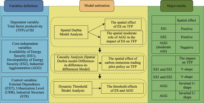
The spatial spillover effect of energy insecurity on total factor productivity in the iron and steel industry, as well as the potential moderating role of industrial agglomeration, remains poorly understood. This study investigated the spatial spillover effect of energy security on total factor productivity and the moderating role of industrial agglomeration in the relationship between energy security and total factor productivity in the iron and steel industry. Panel data from 24 provinces in China spanning the years 2010 to 2019 were used for this analysis. The research findings demonstrate a positive spatial spillover effect of energy security on total factor productivity, which displays a distinct pattern of attenuated spatial spillover effects. Moreover, evidence from quasi-natural experiments shows a negative spillover effect on total factor productivity when using the energy security-policy interaction term, highlighting the significant impact of policy factors on total factor productivity. Threshold effect tests reveal a “strong-weak” V-shaped trend in the impact of energy security with the increase of industrial agglomeration levels. In addition, this study found an inverted U-shaped relationship between energy security and the impact of industrial agglomeration, suggesting that enhancing energy security contributes to the growth of total factor productivity in the iron and steel industry. The ultimate objective of this research is to provide valuable policy recommendations to the government for ensuring energy security and promoting the sustainable growth of total factor productivity in the iron and steel industry.

Cite this article

SUN Xiaojie , GE Zehui , Guo Zhiyuan . The Spatial Spillover Effect of Energy Insecurity on the Total Factor Productivity of the Iron and Steel Industry: Does Industrial Agglomeration Matter?[J]. Journal of Resources and Ecology, 2025 , 16(2) : 387 -401 . DOI: 10.5814/j.issn.1674-764x.2025.02.009

1 Introduction

The issue of energy insecurity garners significant attention from both practitioners and academics. Expediting the establishment of an accessible and sustainable energy system is paramount for capturing the strategic commanding heights of the energy revolution and safeguarding the long-term interests of the nation. Various factors, such as economic globalization, regional conflicts, the transition toward green energy, and structural imbalances, have contributed to the mounting pressure on the energy supply and demand disparities. Energy security (ES) constitutes one of the three dimensions assessed in the global energy trilemma (Šprajc et al., 2019). Despite the pervasive uncertainties in energy markets, governments have intensified their focus on enhancing energy security. Recent years have witnessed notable achievements in managing energy insecurity across multiple countries (Hasan et al., 2021; Taherzadeh et al., 2021).
China’s burgeoning economy and expanding energy requirements are poised to propel the demand for energy to new heights. However, the growth in energy production capacity is unlikely to keep pace with escalating energy consumption, which would result in a protracted period of energy insecurity. Given the inherent risks associated with energy insecurity and the unique significance of fossil fuels, effective energy management is of paramount importance in the realm of manufacturing production (Suganthi and Samuel, 2012).
The energy security of a nation plays a pivotal role in sustaining its domestic industrial production (Zhang et al., 2021; Mišík, 2022). Among various sectors, the iron and steel industry (ISI) consistently ranks as the foremost energy consumer, accounting for a substantial 13.4% of the total energy consumption in 2019, resulting in approximately 1.938 billion t of carbon emissions. Consequently, selecting the ISI as the research focal point offers a representative and insightful perspective. Assessing the total factor productivity (TFP) of the ISI provides a comprehensive measure of the overall production efficiency of its constituent elements. However, few studies have used spatial panel models for exploring the impact of energy security on TFP, indicating a critical research gap in the existing literature.
The role of industrial agglomeration in the relationship between energy security and total factor productivity is complex. Azari et al. (2016) argued for its positive impact on manufacturing productivity, while Lan et al. (2021) suggested that the “crowded effect” of agglomeration leads to external diseconomies and hampers total factor productivity growth. The existing literature primarily focuses on energy insecurity factors, while neglecting the exploration of the spatial effects of energy insecurity on total factor productivity and the potential moderating role of industrial agglomeration (AGG).
The study makes three main contributions. First, it introduces an influential mechanism to evaluate the spatial spillover and the moderating role in the impact of ES on the TFP of the ISI. Second, it assesses the geographic boundaries of the spatial spillover. Third, it examines whether there is a threshold effect on the impact of ES and investigates whether changes in ES are responsible for the inverted U-shaped effect of AGG on TFP.

2 Literature review and research hypotheses

Scholars have devoted considerable attention to enhancing energy security levels and promoting the sustainability of the iron and steel industry as means to bolster the country’s competitiveness (Ma et al., 2002; Movshuk, 2004; He et al., 2013; Na et al., 2022). However, few have explored the spatial spillover effect of energy insecurity on total factor productivity or the role played by industrial agglomeration in this relationship.

2.1 Direct effect of energy insecurity on total factor productivity

Assuring the ISI chain’s smooth operation hinges on the advancement of energy security within both domestic and neighboring contexts. Neighboring countries serve as external suppliers of fossil energy security and can collaborate with the domestic energy market to establish stability in energy prices and supply (Maltby, 2013).
Energy insecurity detrimentally affects the profitability and production costs of the ISI. Industry growth inherently entails a surge in energy demand (Shahbaz and Lean, 2012). However, when energy insecurity is high, energy prices escalate, taking a severe toll on the profitability and productivity of energy enterprises (Rentschler and Kornejew, 2017). In these circumstances, coal-based fossil energy producers begin to explore alternative energy sources, which often come at a higher cost, thereby amplifying the production expenses of energy-intensive industries (Komal and Abbas, 2015). Moreover, production delays caused by energy interruptions further elevate production costs, impeding the growth of total factor productivity of the ISI. Conversely, consistent electricity consumption fosters sustained improvements in enterprise profitability and productivity (Xu et al., 2022).
Energy insecurity exhibits regional disparities. Studies by both Ofosu-Peasah et al. (2021) and Le and Park (2021) revealed the imbalanced nature of energy insecurity across regions. Gong et al. (2021) employed the entropy weight method to assess energy security in China spanning the period from 2004 to 2017. Their findings indicated a progressive upsurge in energy security, and the three provinces boasting the highest levels of energy security were those endowed with abundant coal resources. Notably, energy security constitutes a pivotal component of energy sustainability, as stipulated by Hou et al. (2021). Hou’s analysis of energy sustainability across China’s 30 provinces revealed significant disparities in its attainment.
Energy consumption exhibits heterogeneous and nonlinear impacts on total factor productivity. Gao et al. (2021) employed the global Malmquist-Luenberger index to measure China’s provincial total factor productivity and found region-specific heterogeneity in the impact of fossil fuel consumption on total factor productivity. Similarly, Zhao et al. (2022) used the same method to assess productivity in the high coal-fired industry. Their findings indicated a U- shaped relationship between coal consumption and high coal-fired industry productivity, while neighboring provinces exhibit an inverted U-shaped correlation.
Due to transportation costs, path dependence in enterprise cooperation, and policies restricting production, the spatial spillover effects of energy insecurity on total factor productivity may exhibit regional boundaries. An increase in geographic distance reduces opportunities for face-to-face communication, amplifies transportation costs, and hampers the efficiency of information transmission (Autant-Bernard and LeSage, 2011), thereby establishing a spatial attenuation boundary for the impact of energy insecurity on total factor productivity. When engaging in innovation activities, firms are more inclined to collaborate with their local counterparts rather than nonlocal ones (He et al., 2018), introducing limitations based on geographical distance for spillover effects. Therefore, this study proposes H1:
H1: Energy insecurity has a spatial spillover effect on the total factor productivity of the ISI, and this spillover has geographic boundaries with spatial attenuation characteristics.

2.2 Moderating role of industrial agglomeration

The phenomenon of industrial agglomeration entails a non-linear relationship between the acquisition and sharing of energy and the production behavior of the ISI. The transformation and upgrading of the industrial structure inevitably give rise to industrial agglomeration, generating an environment conducive to enhanced competitiveness (Cainelli and Ganau, 2018). Consequently, the ISI undergoes a transition from isolated points to spatial clusters in the form of lines or blocks, leading to spatial agglomeration and the emergence of scale effects (Cainelli and Iacobucci, 2009; Jang et al., 2017). As a result, the optimization of the ISI requires the implementation of strategic agglomeration optimization techniques (Cainelli et al., 2006; Antonietti and Cainelli, 2011). While the availability of energy resources and cooperative relationships within these clusters supports the development of specialized products and services in energy-intensive industries (Lamin and Livanis, 2013), variations in the impact of energy security are evident across different levels of industrial agglomeration. With an increasing level of industrial agglomeration, the demand for technological upgrading intensifies, thereby alleviating the constraints imposed by energy on ISI production. Notably, the advancement of digital technology leads to the proliferation of information access channels and a reduction in energy costs, consequently diminishing the significance of local communication (Liu et al., 2022).
Moreover, the presence of energy insecurity can trigger a transition from the agglomeration effect to the crowding effect within industrial dynamics. In the academic discourse on the impact of industrial agglomeration on production efficiency, two primary divergent perspectives have emerged. One perspective posits that the scale effect and technology spillover effect arising from industrial agglomeration can enhance energy utilization and production efficiency (Guo et al., 2020). Conversely, an opposing viewpoint asserts that industrial agglomeration engenders a crowding effect, resulting in escalating unit production costs and a consequent reduction in production efficiency (Brakman et al., 1996). The process of industrial agglomeration amplifies the persistent expansion of production scale and output, consequently heightening the demand for energy resources (Verhoef and Nijkamp, 2002). In regions characterized by low levels of energy security, enterprises experience greater motivation to develop and implement energy-saving technologies, thereby bolstering energy efficiency. This improvement in energy efficiency, attributed to the “energy rebound effect”, leads to a decline in energy prices, prompting production to substitute more costly labor and capital inputs with more economical energy resources (Lin and Zhao, 2016). This observation underscores the notion that in regions with low energy security, industrial agglomeration drives the growth of total factor productivity within the ISI. However, when the carrying capacity of facilities and social services exceeds its limits, resulting in technological lock-in, industrial agglomeration assumes a detrimental role. Consequently, the following hypotheses emerge from this discourse:
H2: Industrial agglomeration exerts a negative moderating influence on the relationship between energy security and total factor productivity.
H3: A threshold effect of industrial agglomeration exists in the relationship between energy security and total factor productivity, while simultaneously a threshold effect of energy security manifests between industrial agglomeration and total factor productivity.
In conclusion, the global energy crisis represents an urgent issue that demands immediate attention and resolution (Rao et al., 2019). As the world’s leading energy consumer and carbon emitter, China finds itself in a crucial transitional period as it continues toward achieving high-quality development and must prioritize the coordinated advancement of its energy sector (Zhu et al., 2021). Due to the substantial reliance of the ISI on fossil fuels, energy insecurity imposes constraints that have the potential to significantly hinder overall productivity. The existing scholarly literature primarily focuses on two key aspects: the assessment of energy insecurity and its influencing factors, and the analysis of spatial heterogeneity in the total factor productivity of the ISI and its underlying determinants. However, the intricate spatial spillover effects of energy insecurity on total factor productivity remain poorly understood. To address this critical knowledge gap, our study diligently examined the spatial spillover effects of energy insecurity on the total factor productivity of the ISI. Moreover, the existing literature has not adequately explored the potential moderating role played by industrial agglomeration and has failed to investigate the associated threshold effect. Consequently, this study meticulously investigated the threshold effect between energy security and total factor productivity (Figure 1).
Figure 1 The research framework of this study

3 Methodology and data

3.1 Econometric methodology

3.1.1 Spatial Durbin model (SDM)

3.1.1.1 The design of the SDM

This study employed a spatial Durbin model:
$\begin{align} & \ln TFPit=\rho \sum\limits_{j=1j\ne i}^{N}{Wijt\ln TFP}it+\beta 0+\beta 1\ln ESIit+ \\ & \beta 2\ln AGGit+\beta 3\sum\limits_{j=1j\ne i}^{N}{Wijt}\ln ESIit+ \\ & \beta 4\sum\limits_{j=1j\ne i}^{N}{Wijt\ln AGGit+\sum\limits_{k=1}^{3}{\delta kCkit+}}\mu i+ \\ & \ \nu t+\varepsilon it \end{align}$
where spatial units (provinces) are indexed by i, j, ij (i, j =1,…, N), and time is indexed by t (t=1, …,T). $\mu i$ and $\nu t$ indicate the individual effects and time effects, respectively. $\beta i$ is the coefficient of the explanatory variable; $\varepsilon it$ is the idiosyncratic error, and we assume that the errors ($\varepsilon it$) are independent and co-distributed. lnTFPit indicates the total factor productivity of the ISI, and lnESIit is the energy security. $Ckit$ represents all control variables, including foreign dependence ($\ln EXTit$), urbanization level ($\ln URBit$), and industrial structure ($\ln STRit$); W is a spatial weight matrix; and $\rho $ is the spatial lag coefficient of the dependent variable.
To verify the moderating role of industrial agglomeration, the spatial moderating model was developed:
$\begin{align} & \ln TFPit=\rho \sum\limits_{j=1j\ne i}^{N}{Wijt\ln TFP}it+\beta 0+\beta 1\ln ESIit+ \\ & \ \beta 2\ln AGGit+\beta 3(\ln ESIit\times \ln AGGit)+ \\ & \ \beta 4\sum\limits_{j=1j\ne i}^{N}{Wijt}\ln ESIit+\beta 5\sum\limits_{j=1j\ne i}^{N}{Wijt\ln AGGit+} \\ & \ \sum\limits_{k=1}^{3}{\delta kCkit+}\mu i+\nu t+\varepsilon it \end{align}$
where lnAGGit is industrial agglomeration, lnESIit×lnAGGit is an interactive term, and $\beta i$ and $\delta k$ are coefficients.

3.1.1.2 Construction of the spatial weight matrix

The adjacency matrix is a 0-1 matrix. When two provinces are adjacent, the corresponding element in the weight matrix is assigned a value of 1; otherwise, it is set to 0. To construct a geographical distance weight matrix, the reciprocal of the spherical distance between the geographic centers of the two provinces is calculated and utilized. The economic weight matrix can be expressed as follows:
$Eij=\frac{1}{\left| \overline{yi}-\overline{yj} \right|},\begin{matrix} {} & (i=j, {{E}_{ii}}=0) \\\end{matrix}$
$\overline{{{y}_{i}}}=\frac{1}{T-{{T}_{0}}+1}\times \sum\limits_{t={{T}_{0}}}^{T}{{{y}_{it}}}$
where yit is the per capita real GDP of province i in year t.

3.1.2 Spatial difference-in-difference-in-differences (SDM-DDD) model

This study employed a comparative exogenous quasi- experimental approach using the carbon emission trading pilot as the basis for establishing a causal relationship between ES and TFP. However, the spatial spillover effect of ES challenges the assumption of the difference-in-differences (DID) model, which assumes no interaction between the treatment and control groups. Consequently, the DID model is not suitable in this context. To address this issue, we introduced a spatial Durbin model with differences-in-differences-in-differences (SDM-DDD) framework that incorporates a spatial spillover term and fixes the “distance variable” in a spatiotemporal manner. By employing the SDM-DDD model, we examined the indirect effects of the pilot policy. This framework not only accounts for spatial correlation but also leverages the advantages of SDM in decomposing spatial effects. To test the indirect effects, we constructed Eq. (5):
$\begin{align} & \ln TFPit=\rho \sum\limits_{j=1j\ne i}^{N}{Wijt\ln TFP}it+\beta 0+\beta 1(\ln ESIit\times \\ & \ Policyit)+\beta 2\ln AGGit+\beta 3\sum\limits_{j=1j\ne i}^{N}{Wijt\times } \\ & \ (\ln ESIit\times Policyit)+\beta 4\sum\limits_{j=1j\ne i}^{N}{Wijt\ln AGGit+} \\ & \ \sum\limits_{k=1}^{3}{\delta kCkit+}\mu i+\nu t+\varepsilon it \end{align}$
where $\ln ESIit\times Policyit$ on the right side is the interactive term of the DDD variable that reflects the implementation of the carbon emissions trading pilot policy. If province i is in the treatment group, $Policyit$ before the advancement of the pilot is equal to 0, and $Policyit$ after the implementation is equal to 1. $\sum\limits_{j\ne i}^{N}{Wijt\times (\ln ESIit\times }Policyit)$ is the spatial lag term of $\ln ESIit\times Policyit$, and $\beta 3$ is its parameter.
Parallel trend tests can validate the suitability of policy analysis employing the SDM-DDD. To assess the parallel trends assumption, we introduced a time classification variable and derived Eq. (6):
$\begin{align} & \ln TFPit=\sum\limits_{k=1}^{p}{\alpha kD_{it}^{T-p}}+\sum\limits_{s=1}^{l}{\alpha sD_{it}^{T+s}}+ \\ & \ \sum\limits_{k=1}^{p}{\rho k\sum\limits_{j=1}^{N}{WijD_{jt}^{T-k}}}+\sum\limits_{s=1}^{l}{\rho s}\sum\limits_{j=1}^{N}{WijD_{jt}^{T+s}}+ \\ & \ \rho 1\sum\limits_{j=1}^{N}{Wij\ln TFPjt+\sum\limits_{k=1}^{3}{\delta kCkit+\mu i+}}vt+\varepsilon it \end{align}$
Eq. (6) is a modification of Eq. (5), where T represents the year when the policy pilot was first launched, $D_{it}^{T+h}\left( h\in \left\{ -p,-p+1,\cdots 0,\cdots,l-1,\left. l \right\} \right. \right)$ is the DDD variable of year T + h, and p and l are the maximum time distances before and after the pilot was launched. If province i launched the pilot in year T+h, then $D_{it}^{T+h}=\ln ESIit$; otherwise, $D_{it}^{T+h}$ = 0. This study used T = 2015 as the base period (so $D_{it}^{T}$ is not included in Eq. (6)), and p = l = 4 makes the lengths of the periods before and after the base period equal, to test whether the parallel trend hypothesis is tenable based on the indirect effect of $D_{it}^{T+k}$.

3.1.3 Dynamic panel threshold model (DPTR)

To unveil the intricate dynamics underlying the moderating role of industrial agglomeration, this study employed a DPTR model, building upon the advancements made by Seo et al. (2019) in tracking changes in the coefficients of core explanatory variables. This novel modeling approach offers notable advantages over the panel threshold model proposed by Hansen (1999) and Dang et al. (2012). The DPTR model can be formulated as follows:
$\begin{align} & \ln TFPit=\beta 0+\beta 1\ln TFPit-1+\beta 2\ln ESIit\times \\ & \ \ \ \ \ \ \ \ \ \ \ \ \ I(\ln AGGit\le q)+\beta 3\ln ESIit\times \\ & \ \ \ \ \ \ \ \ \ \ \ \ \ I(\ln AGGit>q)+\sum\limits_{k=1}^{3}{\delta kCkit+} \\ & \ \ \ \ \ \ \ \ \ \ \ \ \ \mu i+\nu t+\varepsilon it \\ \end{align}$
where $\ln TFPit-1$ is the one lag total factor productivity.
The impact of industrial agglomeration on total factor productivity can exhibit divergent patterns depending on the various levels of energy security across different regions. To comprehensively investigate this phenomenon, a DPTR model was constructed:
$\begin{align} & \ln TFPit=\beta 0+\beta 1\ln TFPit-1+\beta 2\ln AGGit\times \\ & \ \ \ \ \ \ \ \ \ \ \ \ \ \ I(\ln ESIit\le q)+\beta 3\ln AGGit\times \\ & \ \ \ \ \ \ \ \ \ \ \ \ \ \ I(\ln ESIit>q)+\sum\limits_{k=1}^{3}{\delta kCkit+} \\ & \ \ \ \ \ \ \ \ \ \ \ \ \ \ \mu i+\nu t+\varepsilon it \\ \end{align}$
where q represents the specific threshold value, and I() is the indicator function.

3.2 Variables and data sources

3.2.1 Total factor productivity (TFP)

In this study, the Super slack-based measure method (Super-SBM) developed by Tone (2001) was employed to measure the total factor productivity of the ISI. As shown in Table 1, input-output indicators were used to calculate the TFP, drawing on the works of Feng et al. (2021) and Wen and Jia (2022).

3.2.2 Energy insecurity (EI)

Inspired by the methodology employed by Le and Park (2021), this study adopted a dimension-based approach and selected two indicators that emphasize scientific rigor: 1) Energy production/energy consumption; and 2) CO2 emission intensity (thousand tons of CO2 emissions per 100 million yuan of GDP in 2009 at purchasing power parity (PPP)). The first indicator represents the measure of energy security availability, capturing the physical accessibility of energy resources such as coke, gasoline, diesel, and electricity, which are all converted into standard coal equivalents based on their calorific values. The second indicator gauges the potential for energy security development, offering insights into its expandability and adaptability.

3.2.3 Industrial agglomeration (AGG)

As discussed by Han et al. (2022), the location quotient serves as an estimation tool for assessing the degree of industrial agglomeration within the ISI. A higher location quotient value indicates a greater level of industrial agglomeration within the respective region.
$L{{Q}_{j}}=\frac{{{{p}_{ij}}}/{{{p}_{j}}}\;}{{{{p}_{i}}}/{p}\;}$
where $LQj$ is the location quotient; pij represents the employment of the i industrial sectors in the j region; pj is the employment of the whole industrial sector in the j region; pi denotes the employment of the i industrial sector, and p is the employment of the whole industrial sector in all regions.

3.2.4 Control variables

Building upon the works of Wong (2009), Drucker and Feser (2012), and Zhao et al. (2022), we acknowledge that TFP can be influenced by various factors. For a comprehensive understanding, Table 1 presents the definitions of the variables used in this study, with all data collected at the provincial level.
Table 1 Statistical descriptions of the variables
Type Variable Definition Calculation method Unit
Variables for
measuring TFP
input 1 Asset investment Net value of fixed assets of the ISI by region billion yuan
input 2 Number of employees Average number of employees of the ISI by region 10 thousand
people
input 3 Intermediate input Operating costs+Operating expenses+Administrative expenses+Finance charges-Salaries-Depreciation expenses billion yuan
output Operating revenue Operating revenue of the ISI by region billion yuan
Variables for
regressions
TFP Total factor productivity Composite scores calculated by the Super-SBM model -
ES1 Energy security 1 (ES1) (availability of
energy security)
Energy production/Energy consumption
(A higher index indicates a higher level of energy security)
-
ES2 Energy security 2 (ES2) (developability of
energy security)
Carbon emissions/GDP kt per billion
yuan
AGG Industrial agglomeration (AGG) Degree of ISI agglomeration measured by location quotient -
EXT External dependence Proportion of total import and export trade value in GDP %
URB Urbanization level Proportion of urban population to permanent population %
STR Industrial structure Proportion of the added value of the secondary industry locally to the added value of the secondary industry in all regions %

3.2.5 Data sources

The data were sourced from the China Industrial Statistical Yearbook, China Economic Census Yearbook, China Energy Statistical Yearbook, Wind database, and provincial statistical yearbooks. This study analyzed a data set from 24 provinces (excluding Beijing, Shanxi, Chongqing, Guizhou, Yunnan, Xizang, Hong Kong, Macao, Hainan, and Taiwan) during 2010-2019. Taking 2009 as the base period, the deflator was used to deflate the GDP. The missing data were filled with linear interpolation. To unify the amount of data and eliminate multicollinearity, this study processed the data logarithmically and then took the zero-centered form.

4 Empirical results and discussion

4.1 Estimation results of the spatial econometric model

4.1.1 Spatial correlation test

Drawing upon the work of Wu et al. (2009), we employed a sophisticated spatial analysis technique to investigate the spatial correlation of TFP. Specifically, the global Moran index, complemented by the LISA index, was applied and integrated with the Bayesian smoothing technique. The findings reveal a significant positive spatial dependence of TFP in both geographical and economic space, as indicated by Moran’s I. To visually represent these results, Figure 2 presents the EB-based Moran’s I values and their corresponding levels of significance.
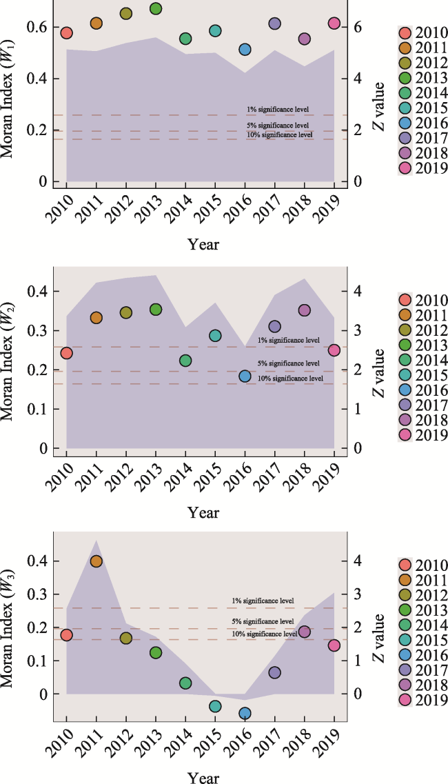
Figure 2 Moran’s I Test results under different spatial weights matrices
Note: The scatter plot illustrates the temporal dynamics of the Moran’s Index across the observation period. The area chart delineates the corresponding Z values.
Table 2 presents the provinces categorized by their respective spatial association types, as determined by the LISA agglomeration index. The spatial agglomeration of TFP is closely linked to the government’s macroeconomic control measures and technological advancements. Shanghai, with its early adoption of cutting-edge technologies like artificial intelligence, the industrial Internet, and the government’s strategic cost reduction initiatives, enjoys a distinct first-mover advantage. Macrocontrol policies have facilitated the transfer of industrial structure innovation to the western and northeastern regions. However, compared to Shanghai, these regions face major challenges such as limited innovation and development momentum, lower energy efficiency per unit of production, and constrained regional capacity, resulting in a pattern of low-low agglomeration. Conversely, the northeastern region is capitalizing on the emerging opportunities of digital manufacturing within the industrial structure, leading to a high-low agglomeration pattern.
Table 2 Spatial agglomeration pattern of the TFP annual mean under each weight matrix
Spatial correlation type Geographic adjacency matrix (W1) Geographic weight matrix (W2) Economic weight matrix (W3)
High-high agglomeration Hebei, Tianjin, Liaoning (3) Inner Mongolia, Jilin, Liaoning (3) Shanghai (1)
Low-high agglomeration None (0) Shandong (1) None (0)
Low-low agglomeration Xinjiang, Qinghai, Gansu, Sichuan, Shaanxi (5) Xinjiang, Qinghai, Gansu, Sichuan, Guangxi, Hunan (6) Xinjiang, Qinghai, Shaanxi, Sichuan, Hubei, Guangxi, Hunan, Anhui, Gansu, Jiangxi, Chongqing (11)
High-low agglomeration None (0) None (0) Heilongjiang, Jilin, Liaoning, Hebei (4)

Note: The number of provinces under each agglomeration type is given in parentheses.

4.1.2 Estimated results of the direct effect

The selection of a suitable spatial econometric model is essential. The results of the LR test and the Wald test indicated that the SLM (Spatial Lag Model) and SEM (Spatial Error Model) should not be adopted. Furthermore, the coefficients of the spatial lag terms in the model were found to be significant at the 1% level, suggesting that the SDM with a space-time bi-fixed effect is the appropriate choice.
Table 3 demonstrates the positive spillover effects of ES1 and ES2. Note that ES1 exhibits a positive spillover effect in geographically adjacent provinces and close areas. Similarly, ES2 shows a positive spillover effect on TFP in geographically adjacent provinces, close areas, and regions with similar economic growth.
Table 3 Direct effect estimation results of the SDM
Variable Spatial Durbin Models
Geographic adjacency matrix (W1) Geographic weight matrix (W2) Economic weight matrix (W3)
(1) (2) (3) (4) (5) (6)
lnES1 0.1722**
(2.42)
- 0.5127***
(5.97)
- 0.1594**
(2.36)
-
lnES2 - 0.0609
(1.42)
- 0.1169***
(2.63)
- 0.0139
(0.34)
lnAGG 0.0606**
(1.96)
0.0384
(1.35)
0.0607**
(2.33)
0.0184
(0.68)
0.1294***
(4.37)
0.1217***
(4.11)
lnAGG 0.0441
(0.78)
-0.0143
(-0.24)
-0.5683***
(-2.80)
-0.6198***
(-2.70)
0.0423
(0.70)
0.0347
(0.65)
lnES1 0.3379**
(2.13)
- 3.2065***
(5.23)
- 0.1725
(0.88)
-
lnES2 - 0.2426**
(2.28)
- 1.5205***
(4.02)
- 0.2743**
(1.96)
Control variables Control Control Control Control Control Control
$\rho $ -0.4070***
(-4.71)
-0.4270***
(-4.96)
-1.4006***
(-5.76)
-1.2676***
(-5.13)
-0.2898***
(-3.47)
-0.2768***
(-3.29)
R2 0.4132 0.4108 0.4550 0.3953 0.3472 0.3397
Log-likelihood -3.3734 -4.4043 0.0086 -10.6073 -13.4001 -14.5206

Note: Figures shown in parentheses are T values. *P < 0.1, **P < 0.05, ***P < 0.01.

Two factors contribute to the positive spatial spillover effect of ES on TFP in the ISI. First, ES1 acts as a catalyst for ISI development, facilitated by energy allocation projects like the West-East Gas Pipeline which address diverse energy endowments (Gong et al., 2021). Stable ES1 enables green energy transformation and industrial symbiosis, thereby improving production capacity utilization and enhancing TFP. Second, natural factors like wind direction and topography influence ES2, leading to spatial dependence and CO2 diffusion to surrounding areas (Meng et al., 2017). Consequently, the surrounding provinces naturally become transfer and radiation areas for ES2, further contributing to the positive spatial spillover effect on TFP in the steel industry.

4.1.3 Estimation results of decomposition effects

Based on the partial differential estimation results and further analysis (Autant-Bernard and LeSage, 2011) (Table 4), the indirect effects can be described as follows. A 1% increase in ES1 yields a 0.2199% increase in TFP for adjacent provinces, while a 1% increase in ES2 corresponds to a 0.1722% increase. Geographically close areas experience a substantial 1.2036% TFP increase for every 1% rise in ES1, and a notable 0.6808% increase for every 1% rise in ES2. Provinces with similar economic growth witness a modest 0.1455% TFP increase for every 1% rise in ES2. However, the spatial spillover coefficient of ES1 under W3 shows no statistical significance. Notably, the coefficient of ES under W2 exhibits the largest absolute value, highlighting the significant contribution of regional ES to TFP growth in geographically close areas.
Table 4 Estimation results of SDM’s decomposition effects
Variable Geographic adjacency matrix (W1) Geographic weight matrix (W2) Economic weight matrix (W3)
Direct effect Indirect effect Total effect Direct effect Indirect effect Total effect Direct effect Indirect effect Total effect
lnES1 0.1446*
(1.94)
0.2199*
(1.65)
0.3645***
(2.98)
0.3675***
(4.54)
1.2036***
(3.92)
1.5710***
(5.00)
0.1477**
(2.08)
0.1040
(0.63)
0.2517*
(1.64)
lnES2 0.0370
(0.81)
0.1722*
(1.86)
0.2092***
(2.65)
0.0451
(0.97)
0.6808***
(3.54)
0.7259***
(3.77)
0.0021
(0.05)
0.1455**
(1.99)
0.1476**
(1.99)

Note: Figures shown in parentheses are T values. *P < 0.1, **P < 0.05, ***P < 0.01.

4.1.4 Attenuation boundaries of the spatial spillover effects

The geospatial distance threshold matrices were calculated as follows:
${{W}_{4}}=\left\{ \begin{align} & \frac{1}{dij},dij>dthre \\ & 0,\begin{matrix} {} \\\end{matrix}dij\le dthre \\ \end{align} \right.$
where $dij$ refers to the shortest traffic distance between the cities and $dthre$ refers to the given distance threshold.
${{W}_{5}}=\left\{ \begin{align} & \frac{1}{di{{j}^{2}}},\ dij>dthre \\ & 0,\begin{matrix} {} \\\end{matrix}\ \ dij\le dthre \\ \end{align} \right.$
where dij2 represents the square of the geographic distance.
Figure 3 illustrates the variation in the ES coefficients with geographical distance. The spatial spillover coefficients show significance within two radii: approximately 0- 200 km and 400-600 km. Specifically, when the distance threshold is less than 200 km, ES exhibits a polarization effect on the TFP in adjacent areas. However, within the 200-400 km radius, ES does not demonstrate a significant spatial spillover effect. This can be attributed to the closer proximity to areas with a high level of energy security, leading to a stronger dependence of their ISI on fossil energy, enhanced division of labor, cooperation in the production process, and reduced resource acquisition costs. Notably, the spatial spillover coefficients of ES1 and ES2 are not significant within the 200-400 km radius, while the negative coefficient becomes significant near the threshold of 400-600 km. This indicates an inhibitory effect of ES within the 400-600 km threshold. One possible explanation is that the substantial increase in energy transportation costs acts as a hindrance to TFP growth. However, beyond 600 km, no significant spillover effect is observed.
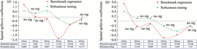
Figure 3 Variation in the energy insecurity spatial spillover coefficients with geographic distance (a) SDM estimation using W4; (b) SDM estimation using W5

Note: Regression using W4 served as the benchmark regression for Eq. (1), while regression with W5 for Eq. (1) was employed as the robustness test.

4.1.5 Estimated causality results

The carbon emissions trading pilot policy has significantly affected the TFP of the ISI, enhancing its international competitiveness in the low-carbon sector (Qi et al., 2021). In the pilot cities, companies received greenhouse gas emission quotas for a specific period, leading to an effective improvement in TFP (Tian et al., 2023). This improvement can be attributed to two key factors: the policy’s stimulation of research and development investments and technological innovation by enterprises, and its positive impact on the power generation technology structure (Lai and Chen, 2023; Liu and Liu, 2023).
Table 5 shows the spatial spillover effects of carbon trading pilot programs on the TFP of neighboring regions. Model (8) and (11) reveal negative spatial spillover coefficients that exhibit statistical significance, which underscores the significant negative impact of these carbon trading pilots on the TFP of geographically proximate areas. However, it is noteworthy that upon introducing control variables into the analysis, the interaction term between the Policy and ES2 remains statistically significant, whereas the interaction term between the Policy and ES1 loses its significance. The pervasive “rebound effect” of energy may contribute to diminishing the significance of ES1’s influence on the TFP of the ISI.
Table 5 Causality estimation results of the SDM-DDD models.
Variable SDM-DDD estimation results under the distance spatial weight matrix (W2)
(7) (8) (9) (10) (11) (12)
lnAGG - -0.4346***
(-5.92)
-0.4077**
(-5.28)
- -0.4311***
(-5.91)
-0.4034***
(-5.27)
D.E._lnES1×Policy -0.0107
(-0.06)
0.1396
(0.72)
0.1326
(0.71)
- - -
I.E._lnES1×Policy -2.7776**
(-2.54)
-0.8258
(-1.24)
-0.7561
(-0.99)
- - -
T.E._lnES1×Policy -2.7883**
(-2.50)
-0.6862
(-1.02)
-0.6235
(-0.84)
- - -
D.E._lnES2×Policy - - - 0.0447
(0.62)
0.1048*
(1.65)
0.1375**
(2.00)
I.E._lnES2×Policy - - - -1.100***
(-3.26)
-0.4155**
(-1.99)
-0.3021
(-1.10)
T.E._lnES2×Policy - - - -1.0553*
(-3.00)
-0.3107
(-1.48)
-0.1647
(-0.57)
Control variables No control No control Control No control No control Control
$\rho $ -0.3296
(-1.56)
-0.8926***
(-3.70)
-0.9776***
(-3.99)
-0.3576*
(-1.68)
-0.8536***
(-3.55)
-0.9186***
(-3.78)
R2 0.6919 0.7470 0.7521 0.6992 0.7438 0.7541
Log-likelihood 78.7993 98.3216 99.8913 81.5653 97.4650 101.45276

Note: Figures shown in parentheses are T values. *P < 0.1, **P < 0.05, ***P < 0.01. D.E. before a variable symbol indicates a direct effect, I.E. indicates an indirect effect, and T.E. indicates a total effect.

Since 2013, carbon emission trading pilots have been implemented in eight provinces and cities: Beijing, Shanghai, Tianjin, Chongqing, Hubei, Guangdong, Shenzhen, and Fujian. In this study, the year 2015 was selected as the policy’s inception point, accounting for the inherent time lag between policy formulation and its actual implementation (Meng et al., 2022).
Figure 4 presents a visual representation of the spatial spillover coefficients, accompanied by the upper and lower bounds of the 95% confidence intervals for Policy×ES1, as well as Policy×ES2. Notably, the estimated coefficients are negative during the period 2010-2013 and gradually approach values close to zero in 2014, but they fail to pass the significance test. These observations indicate that prior to policy implementation, no significant disparity is observed between the pilot and non-pilot provinces, thus satisfying the conditions required for parallel trends.
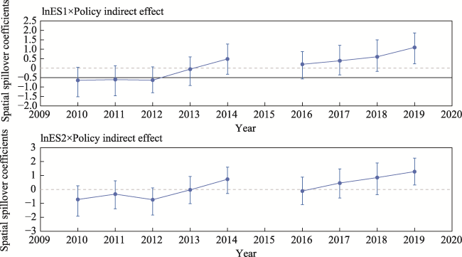
Figure 4 Parallel trend test results of the SDM-DDD model

Note: The gap in the curve is because the base period (2015) was not included in the parallel trend test.

4.1.6 Estimated results of the moderating role of AGG

Table 6 shows that the interaction term coefficients between industrial agglomeration and energy security are negative, indicating a weakening effect of energy security with increasing levels of agglomeration. The reason for this could be the insufficient carrying capacity of regional innovation factors, which greatly reduces the positive impact of ES on TFP. Provinces characterized by a high degree of AGG exhibit “free-rider” behavior and are influenced by the “demonstration effect” of energy utilization, resulting in reduced efforts to improve TFP. Additionally, there is a “synergistic effect” in the agglomeration of manufacturing. Clusters can achieve greater profits by using the same energy through external synergy, which reduces the enterprises’ enthusiasm to optimize resource allocation for improving energy efficiency (Ke, 2010).
Table 6 Estimated results of the moderating effect of industrial agglomeration
Variable Spatial Durbin Models
Geographic adjacency matrix (W1) Geographic weight matrix (W2) Economic weight matrix (W3)
(13) (14) (15) (16) (17) (18)
lnES1 0.1416**
(2.11)
- 0.3701***
(3.56)
- 0.0714
(1.03)
-
lnES2 - 0.2107**
(2.52)
- 0.1325***
(2.75)
- 0.0281
(0.68)
lnAGG 0.1161***
(3.95)
0.0812***
(2.93)
0.0860***
(3.34)
0.0250
(0.87)
0.1293***
(4.55)
0.1542***
(4.89)
lnES1×lnAGG -0.5801***
(-6.87)
- -0.4308*
(-3.63)
- -0.4866***
(-5.01)
-
lnES2×lnAGG - -0.1033***
(-2.90)
- -0.0552
(-1.34)
- -0.1586***
(-3.62)
lnAGG -0.1075*
(-1.73)
0.0037
(0.07)
-0.6711***
(-3.42)
-0.6625***
(-2.58)
0.0352
(0.58)
0.1407**
(2.37)
lnES1 0.2973*
(1.94)
- 2.0659**
(2.51)
- 0.1188
(0.62)
-
lnES2 - 0.0618
(0.54)
- 1.4338***
(2.94)
- 0.2054**
(2.36)
Control variables Control Control Control Control Control Control
$\rho $ -0.4319***
(-5.06)
-0.4990***
(-5.89)
-1.3946***
(-5.62)
-1.2236***
(-4.91)
-0.2348***
(-2.76)
-0.2448***
(-2.89)
R2 0.5158 0.4642 0.4998 0.4023 0.4094 0.3723
Log-likelihood 18.8300 4.6596 10.3631 -8.6341 -0.4222 -7.9065

Note: Figures displayed in parentheses are T values. *P < 0.1, **P < 0.05, ***P < 0.01.

4.2 Panel threshold regression results

4.2.1 Estimation results of the dynamic panel threshold model

Table 7 presents the results pertaining to thresholds and their corresponding 90% confidence intervals. The likelihood ratio (LR) graph in Models (20)-(22) shows a smooth and consistent pattern, with the 90% line intersecting the upper and lower boundaries of the confidence intervals. Conversely, the LR plot of Model (19) appears disorganized and lacks the presence of the 90% line, indicating the threshold’s failure to meet the significance test criteria. The SupWStar test yields the same conclusion, thereby confirming the non-significance of the threshold. Therefore, as AGG progressively exceeds a specific threshold, a weakened trend is observed in the negative impacts of both ES1 and ES2 on TFP. Similarly, when either ES1 or ES2 surpasses a certain threshold, an inverted U-shaped effect of AGG on TFP emerges.
Table 7 Threshold values of different threshold variables and their confidence intervals
Model Threshold variables SupWStar Threshold value ES1 value ES2 value AGG value 90% confidence interval
Lower Higher
(19) lnAGG 32.2878
(1.44)
0.2451 - - 0.5233 -0.9059 0.9908
(20) lnAGG 388.8587***
(5.99)
0.2760 - - 0.5397 -0.9059 0.3622
(21) lnES1 223.2055*
(1.64)
0.0918 1.0712 - - 0.0918 0.1100
(22) lnES2 115.6495**
(2.14)
-0.2794 - 13.8461 - -0.3922 0.8191

Note: The parameter estimation of DPTR uses the theory and code provided by Kremer et al. (2013). Figures shown in parentheses are Z values. *P < 0.1, **P < 0.05, ***P < 0.01. The results were evaluated based on 200 replications of regression.

The findings presented in Table 8 reveal the varying influence of energy security across different levels of AGG. Once AGG surpasses the threshold, the positive impacts of ES1 and ES2 on TFP weaken, primarily due to the negative moderating effect of AGG. While the threshold effect in Model (19) using AGG as the threshold variable lacks significance, a notable transformation of ES1’s coefficient is observed at the 1% significance level when AGG exceeds 0.5233 (resulting in a reduction of 0.4071 in the positive effect). Conversely, the threshold effect in Model (20) is statistically significant, with the coefficient of ES2 decreasing by 0.0209.
Table 8 Regression results of dynamic panel threshold models
Variable (19) (20) (21) (22)
lnTFPit-1 0.3230***
(6.01)
0.2843***
(6.43)
0.2921***
(11.13)
0.4598***
(9.16)
lnES1(lnAGG≤c) 1.7297***
(4.94)
- - -
lnES1(lnAGG>c) 1.3226***
(3.41)
- - -
lnES2(lnAGG≤c) - 0.4989**
(2.35)
- -
lnES2(lnAGG>c) - 0.4780***
(3.15)
- -
lnAGG(lnES1≤c) - - 0.3453***
(5.09)
-
lnAGG(lnES1>c) - - -0.3376***
(-3.13)
-
lnAGG(lnES2≤c) - - - 0.1709**
(2.04)
lnAGG(lnES2>c) - - - -0.2053***
(-2.62)
Control variables Control Control Control Control
_cons 0.0350
(0.50)
0.0383
(0.64)
-0.0495
(-0.91)
0.0570
(1.29)
Wald test 362.43
[P=0.0000]
311.81
[P=0.0000]
299.26
[P=0.0000]
635.81
[P=0.0000]
Sargan test 20.33
[P=0.5624]
20.20
[P=0.5704]
21.54
[P=0.4876]
19.58
[P=0.6094]
AR(1) -1.91
[P=0.0557]
-1.74
[P=0.0820]
-2.15
[P=0.0312]
-2.19
[P=0.0285]
AR(2) -0.8605
[P=0.3895]
-0.19
[P=0.8475]
-0.95
[P=0.3446]
-0.42
[P=0.6768]

Note: Figures shown in parenthese are T values, and figures shown in brackets are P values. *P<0.1, **P<0.05, ***P<0.01.

Furthermore, the relationship between AGG and TFP exhibits an inverted U-shaped pattern. In provinces characterized by low ES, AGG positively impacts TFP; conversely, AGG exerts an inhibitory effect in provinces with high ES. Regional variation in the impact of agglomeration on energy efficiency has been validated in studies conducted across diverse industries. For instance, Zheng and Lin (2018) examined the impact of agglomeration in the paper industry using a static threshold panel model and found an inverted U-shaped characteristic. Similarly, Williamson (1965) discovered an inverted U-shaped impact of industrial agglomeration on production efficiency.

4.2.2 Analysis of the phases of the impacts of ES and AGG on TFP

Figure 5 illustrates the phased results based on thresholds for the number of provinces. This study specifically analyzed the years 2010, 2013, 2016, and 2019 as key reference points.
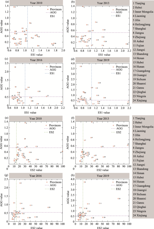
Figure 5 Phased results of the provinces based on threshold values (a-d) the phases of the impacts of ES1 and AGG on TFP; (e-f) the phases of the impacts of ES2 and AGG on TFP

Note: The graphs depict energy security levels on the horizontal axis and industrial agglomeration on the vertical axis. The reference lines for the horizontal axis represent the two energy security threshold values (ES1 and ES2) at 1.0712 and 13.8461, respectively. The reference lines on the vertical axis indicate the dual thresholds for industrial agglomeration at 0.5233 and 0.5397.

The ES1 of each province remains relatively stable, with a declining positive impact on TFP observed across most provinces over time. In 2010, the ES1 was low for most provinces, with AGG values below 0.5233. Some major coal-producing provinces, such as Gansu, Xinjiang, and Shaanxi, exhibited relatively high ES1 due to increased energy consumption and production constraints. Conversely, provinces like Hebei, Shanghai, and Tianjin had relatively low ES1 due to their efforts in transitioning toward greener energy sources and exploring alternative energy options. Notably, significant industrial clusters had formed in major steel-producing provinces like Hebei, Liaoning, and Inner Mongolia. During this period, most provinces experienced a phase where ES1 had a stronger positive effect on TFP, with AGG playing a constructive role. By 2013, ES1 and AGG showed limited changes among the provinces. By 2019, the number of provinces with ES1 below 1.0712 remained unchanged, indicating that ES1 had not undergone significant changes due to the transition toward greener energy structures and the exploration of alternative energy sources. AGG continued to play a positive role. Only eight provinces exhibited a greater contribution of ES1 to TFP growth, with only four provinces demonstrating a promoting effect of AGG. The remaining 16 provinces displayed a less pronounced positive effect of ES1 on TFP.
Similarly, the ES2 of provinces remained largely unchanged, with a decreasing positive effect on TFP observed in most provinces over time. In 2010, most provinces exhibited higher ES2 and lower AGG. During this period, ES2 played a more prominent role in promoting TFP growth in most provinces. Except for Shanghai, Guangdong, and Fujian, the other provinces generally experienced high levels of ES2, indicating that AGG had a negative impact on TFP in 87.5% of the provinces. By 2019, the positive effect of ES2 on TFP had weakened in most provinces due to the increasing influence of AGG. Provinces like Zhejiang, Jiangsu, and Hunan saw their ES2 values drop below 13.8461, signifying that AGG had a positive effect on TFP in 54.17% of the provinces. Following the lead of Shanghai and Guangdong, Hunan and Zhejiang entered the third quadrant. These four provinces demonstrated stronger positive effects of ES2 on TFP, with AGG playing a constructive role.
Overall, energy security has a positive impact on total factor productivity during the process of enhancing industrial agglomeration. However, this effect diminishes as agglomeration reaches higher levels. Furthermore, the positive impact of industrial agglomeration can only be realized within a certain range of energy security levels.

5 Conclusions and policy implications

This study presents several key findings. First, ES has a positive impact on the TFP of the ISI. Second, ES exhibits a positive spatial spillover effect on the TFP in neighboring areas, with a discernible spatial attenuation boundary. The energy security of carbon trading pilots negatively affects the TFP in adjacent regions, suggesting that policy plays a significant role in shaping the spatial effect of ES. Third, the positive influence of ES on TFP is weakened by AGG. Fourth, a threshold effect exists, resulting in an inverted V-shaped pattern of the impact of ES on TFP. Moreover, the presence of a threshold effect also implies that the enhancement of ES provides a reasonable explanation for the inverted U-shaped relationship between AGG and TFP.
Based on these findings, we propose the following recommendations. First, governments should adopt and implement policies aimed at continually enhancing energy security. These policies should focus on increasing the proportions of fossil energy production and consumption, facilitating the transition to greener energy sources, and expanding the utilization of renewable energy in the supply chain. Second, fostering a symbiotic relationship between the government and enterprises will drive the growth of TFP through energy security. Governments can establish and improve systems for trading new energy technologies and energy-saving technologies in the market, while actively promoting the development of wind power and photovoltaic bases. Steel enterprises should enhance their production processes and technological innovation, such as transitioning from long-process steel production to short-process methods and adopting green hydrogen steelmaking, in order to explore new avenues for growth. Lastly, governments should delineate the boundaries of local energy security and establish stricter constraints on local industrial agglomeration. To maximize the positive effects of energy security, excessive industrial agglomeration should be avoided. Governments can introduce subsidies for renewable energy or special funds for redistributing revenue to alleviate the capital investment pressures caused by excessive energy consumption and CO2 emissions from companies.
[1]
Antonietti R, Cainelli G. 2011. The role of spatial agglomeration in a structural model of innovation, productivity and export: A firm-level analysis. The Annals of Regional Science, 46: 577-600.

[2]
Autant-Bernard C, LeSage J P. 2011. Quantifying knowledge spillovers using spatial econometric models. Journal of Regional Science, 51(3): 471-496.

[3]
Azari M, Kim H, Kim J Y, et al. 2016. The effect of agglomeration on the productivity of urban manufacturing sectors in a leading emerging economy. Economic Systems, 40(3): 422-432.

[4]
Brakman S, Garretsen H, Gigengack R, et al. 1996. Negative feedbacks in the economy and industrial location. Journal of Regional Science, 36(4): 631-651.

[5]
Cainelli G, Ganau R. 2018. Distance-based agglomeration externalities and neighbouring firms’ characteristics. Regional Studies, 52(7): 922-933.

[6]
Cainelli G, Iacobucci D. 2009. Do agglomeration and technology affect vertical integration? Evidence from Italian business groups. International Journal of the Economics of Business, 16(3): 305-322.

[7]
Cainelli G, Iacobucci D, Morganti E. 2006. Spatial agglomeration and business groups: New evidence from Italian industrial districts. Regional Studies, 40(5): 507-518.

[8]
Dang V A, Kim M, Shin Y. 2012. Asymmetric capital structure adjustments: New evidence from dynamic panel threshold models. Journal of Empirical Finance, 19(4): 465-482.

[9]
Drucker J, Feser E. 2012. Regional industrial structure and agglomeration economies: An analysis of productivity in three manufacturing industries. Regional Science and Urban Economics, 42(1-2): 1-14.

[10]
Feng G H, McLaren K R, Yang O, et al. 2021. The impact of environmental policy stringency on industrial productivity growth: A semi-parametric study of OECD countries. Energy Economics, 100: 105320. DOI: 10.1016/j.eneco.2021.105320.

[11]
Gao Y N, Zhang M C, Zheng J H. 2021. Accounting and determinants analysis of China’s provincial total factor productivity considering carbon emissions. China Economic Review, 65: 101576. DOI: 10.1016/j.chieco.2020.101576.

[12]
Gong X, Wang Y, Lin B Q. 2021. Assessing dynamic China’s energy security: Based on functional data analysis. Energy, 217: 119324. DOI: 10.1016/j.energy.2020.119324.

[13]
Guo Y H, Tong L J, Mei L. 2020. The effect of industrial agglomeration on green development efficiency in Northeast China since the revitalization. Journal of Cleaner Production, 258: 120584. DOI: 10.1016/j.jclepro.2020.120584.

[14]
Han J, Li G X, Shen Z, et al. 2022. Manufacturing transfer and environmental efficiency: Evidence from the spatial agglomeration of manufacturing in China. Journal of Environmental Management, 314: 115039. DOI: 10.1016/j.jenvman.2022.115039.

[15]
Hansen B E. 1999. Threshold effects in non-dynamic panels: Estimation, testing, and inference. Journal of Econometrics, 93(2): 345-368.

[16]
Hasan A S M M, Tuhin R A, Ullah M, et al. 2021. A comprehensive investigation of energy management practices within energy intensive industries in Bangladesh. Energy, 232: 120932. DOI: 10.1016/j.energy.2021.120932.

[17]
He F, Zhang Q Z, Lei J S, et al. 2013. Energy efficiency and productivity change of China’s iron and steel industry: Accounting for undesirable outputs. Energy Policy, 54: 204-213.

[18]
He Z L, Tong T W, Zhang Y C, et al. 2018. A database linking Chinese patents to China’s census firms. Scientific Data, 5(1): 1-16.

[19]
Hou X R, Lv T, Xu J, et al. 2021. Energy sustainability evaluation of 30 provinces in China using the improved entropy weight-cloud model. Ecological Indicators, 126: 107657. DOI: 10.1016/j.ecolind.2021.107657.

[20]
Jang S, Kim J, von Zedtwitz M. 2017. The importance of spatial agglomeration in product innovation: A microgeography perspective. Journal of Business Research, 78: 143-154.

[21]
Ke S Z. 2010. Agglomeration, productivity, and spatial spillovers across Chinese Cities. The Annals of Regional Science, 45(1): 157-179.

[22]
Komal R, Abbas F. 2015. Linking financial development, economic growth and energy consumption in Pakistan. Renewable and Sustainable Energy Reviews, 44: 211-220.

[23]
Kremer S, Bick A, Nautz D. 2013. Inflation and growth: New evidence from a dynamic panel threshold analysis. Empirical Economics, 44(2): 861-878.

[24]
Lai J M, Chen Y Y. 2023. Innovation spillover effect of the pilot carbon emission trading policy in China. Heliyon, 9(9): e20062. DOI: 10.1016/j.heliyon.2023.e20062.

[25]
Lamin A N, Livanis G. 2013. Agglomeration, catch-up and the liability of foreignness in emerging economies. Journal of International Business Studies, 44(6): 579-606.

[26]
Lan F, Sun L, Pu W Y. 2021. Research on the influence of manufacturing agglomeration modes on regional carbon emission and spatial effect in China. Economic Modelling, 96: 346-352.

[27]
Le T H, Park D. 2021. What drives energy insecurity across the world? A panel data analysis. Energy Research & Social Science, 77: 102093. DOI: 10.1016/j.erss.2021.102093.

[28]
Lin B Q, Zhao H L. 2016. Technological progress and energy rebound effect in China’s textile industry: Evidence and policy implications. Renewable and Sustainable Energy Reviews, 60: 173-181.

[29]
Liu J Y, Liu X. 2023. Effects of carbon emission trading schemes on green technological innovation by industrial enterprises: Evidence from a quasi-natural experiment in China. Journal of Innovation & Knowledge, 8(3): 100410. DOI: 10.1016/j.jik.2023.100410.

[30]
Liu Y H, Wu A Q, Song D. 2022. Exploring the impact of cross-side network interaction on digital platforms on internationalization of manufacturing firms. Journal of International Management, 28(4): 100954. DOI: 10.1016/j.intman.2022.100954.

[31]
Ma J L, Evans D G, Fuller R J, et al. 2002. Technical efficiency and productivity change of China’s iron and steel industry. International Journal of Production Economics, 76(3): 293-312.

[32]
Maltby T. 2013. European Union energy policy integration: A case of European Commission policy entrepreneurship and increasing supranationalism. Energy Policy, 55: 435-444.

PMID

[33]
Meng B, Wang J G, Andrew R, et al. 2017. Spatial spillover effects in determining China’s regional CO2 emissions growth: 2007-2010. Energy Economics, 63: 161-173.

[34]
Meng Y L, Wang L, Wei Y G, et al. 2022. Time-frequency dynamics, co-movement and causality among returns of global carbon emissions trading schemes (ETSs): A tale of four markets. Journal of Cleaner Production, 363: 132564. DOI: 10.1016/j.jclepro.2022.132564.

[35]
Mišík M. 2022. The EU needs to improve its external energy security. Energy Policy, 165: 112930. DOI: 10.1016/j.enpol.2022.112930.

[36]
Movshuk O. 2004. Restructuring, productivity and technical efficiency in China’s iron and steel industry, 1988-2000. Journal of Asian Economics, 15(1): 135-151.

[37]
Na H M, Sun J C, Qiu Z Y, et al. 2022. Optimization of energy efficiency, energy consumption and CO2 emission in typical iron and steel manufacturing process. Energy, 257: 124822. DOI: 10.1016/j.energy.2022.124822.

[38]
Ofosu-Peasah G, Ofosu Antwi E, Blyth W. 2021. Factors characterising energy security in West Africa: An integrative review of the literature. Renewable and Sustainable Energy Reviews, 148: 111259. DOI: 10.1016/j.rser.2021.111259.

[39]
Qi S Z, Zhou C B, Li K, et al. 2021. The impact of a carbon trading pilot policy on the low-carbon international competitiveness of industry in China: An empirical analysis based on a DDD model. Journal of Cleaner Production, 281: 125361. DOI: 10.1016/j.jclepro.2020.125361.

[40]
Rao N D, Min J, Mastrucci A. 2019. Energy requirements for decent living in India, Brazil and South Africa. Nature Energy, 4(12): 1025-1032.

DOI

[41]
Rentschler J, Kornejew M. 2017. Energy price variation and competitiveness: Firm level evidence from Indonesia. Energy Economics, 67: 242-254.

[42]
Seo M H, Kim S, Kim Y J. 2019. Estimation of dynamic panel threshold model using Stata. The Stata Journal: Promoting Communications on Statistics and Stata, 19(3): 685-697.

[43]
Shahbaz M, Lean H H. 2012. Does financial development increase energy consumption? The role of industrialization and urbanization in Tunisia. Energy Policy, 40: 473-479.

[44]
Šprajc P, Bjegović M, Vasić B. 2019. Energy security in decision making and governance—Methodological analysis of energy trilemma index. Renewable and Sustainable Energy Reviews, 114: 109341. DOI: 10.1016/j.rser.2019.109341.

[45]
Suganthi L, Samuel A A. 2012. Energy models for demand forecasting—A review. Renewable and Sustainable Energy Reviews, 16(2): 1223-1240.

[46]
Taherzadeh O, Bithell M, Richards K. 2021. Water, energy and land insecurity in global supply chains. Global Environmental Change, 67: 102158. DOI: 10.1016/j.gloenvcha.2020.102158.

[47]
Tian J Z, Liu Y S, Li A L. 2023. The policy impact of carbon emission trading on building enterprises’ total factor productivity in China. Buildings, 13(6): 1493. DOI: 10.3390/buildings13061493.

[48]
Tone K. 2001. A slacks-based measure of efficiency in data envelopment analysis. European Journal of Operational Research, 130(3): 498-509.

[49]
Verhoef E T, Nijkamp P. 2002. Externalities in urban sustainability. Ecological Economics, 40(2): 157-179.

[50]
Wen S Y, Jia Z J. 2022. The energy, environment and economy impact of coal resource tax, renewable investment, and total factor productivity growth. Resources Policy, 77: 102742. DOI: 10.1016/j.resourpol.2022.102742.

[51]
Williamson J G. 1965. Regional inequality and the process of national development: A description of the patterns. Economic Development and Cultural Change, 13(4): 1-84.

[52]
Wong S A. 2009. Productivity and trade openness in Ecuador’s manufacturing industries. Journal of Business Research, 62(9): 868-875.

[53]
Wu P C, Lay J G, Guo H R, et al. 2009. Higher temperature and urbanization affect the spatial patterns of dengue fever transmission in subtropical Taiwan. Science of the Total Environment, 407(7): 2224-2233.

[54]
Xu J, Akhtar M, Haris M, et al. 2022. Energy crisis, firm profitability, and productivity: An emerging economy perspective. Energy Strategy Reviews, 41: 100849. DOI: 10.1016/j.esr.2022.100849.

[55]
Zhang Y J, Li X P, Song Y, et al. 2021. Can green industrial policy improve total factor productivity? Firm-level evidence from China. Structural Change and Economic Dynamics, 59: 51-62.

[56]
Zhao M X, Lv L H, Wu J, et al. 2022. Total factor productivity of high coal-consuming industries and provincial coal consumption: Based on the dynamic spatial Durbin model. Energy, 251: 123917. DOI: 10.1016/j.energy.2022.123917.

[57]
Zheng Q Y, Lin B Q. 2018. Impact of industrial agglomeration on energy efficiency in China’s paper industry. Journal of Cleaner Production, 184: 1072-1080.

[58]
Zhu R M, Zhao R Q, Sun J, et al. 2021. Temporospatial pattern of carbon emission efficiency of China’s energy-intensive industries and its policy implications. Journal of Cleaner Production, 286: 125507. DOI: 10.1016/j.jclepro.2020.125507.

Outlines

/