Ecosystem Quality and Ecosystem Services

Spatio-temporal Dynamics and Drivers of Ecological Quality in Yulin City Using the MRSEI Model

  • MU Weichen , 1, 2, 3, 4 ,
  • HE Zhilin 1, 2, 3, 4 ,
  • CHEN Yanglong 1, 2, 3, 4 ,
  • GAO Dongkai 1, 2, 3, 4 ,
  • YUE Tianming 1, 2, 3, 4 ,
  • QIN Fen , 1, 2, 3, 4, *
Expand
  • 1. College of Geographical Sciences, Faculty of Geographical Science and Engineering, Henan University, Zhengzhou, 450046, China
  • 2. Key Laboratory of Geospatial Technology for the Middle and Lower Yellow River Regions, Ministry of Education, Henan University, Kaifeng, Henan 475004, China
  • 3. Henan Industrial Technology Academy of Spatio-Temporal Big Data, Henan University, Kaifeng, Henan 475004, China
  • 4. Henan Technology Innovation Center of Spatial-Temporal Big Data, Henan University, Zhengzhou 450046, China.
* QIN Fen, E-mail:

MU Weichen, E-mail:

Received date: 2023-12-20

  Accepted date: 2024-05-10

  Online published: 2025-03-28

Supported by

The High-Resolution Satellite Project of the State Administration of Science, Technology, and Industry for National Defense of the PRC(80Y50G19-9001-22/23)

The Major Research Projects of the Ministry of Education(16JJD770019)

The Henan Provincial Key R&D and Promotion Special Project (Science and Technology Research)(242102321122)

The National Natural Science Foundation of China(U21A2014)

Abstract

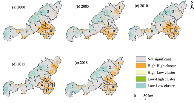
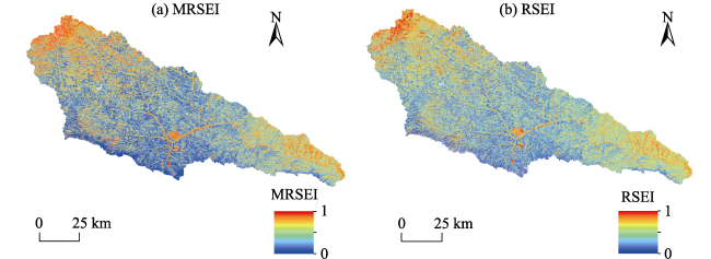
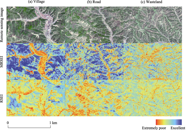
Urbanization has resulted in growing ecological pressures on cities, necessitating assessments of urban ecological quality. Long-term characterization of regional dynamics and drivers is critical for environmental management. This study proposes an enhanced ecological quality model (MRSEI) incorporating vegetation cover and EVI rather than just NDVI. The MRSEI model was applied to analyse ecological quality in Yulin City during 2000-2018 using Landsat TM/OLI data on Google Earth Engine. Geographic detectors also quantified anthropogenic and environmental influences on the study area. The results are summarized as follows: (1) MRSEI showed an average correlation coefficient of 0.840 with other indices, demonstrating higher representativeness than individual components. The principal component analysis indicated a 12.88% increase in explained variance. MRSEI also exhibited significantly improved identification of roads, villages, and unused lands over RSEI, better matching ground conditions, and suitability for regional ecological assessment. (2) During 2000-2020, the average MRSEI in Yulin City was 0.481, peaking at 0.518 in 2018, indicating general ecological improvement over time. Spatially, conditions were better in the southeast than northwest. While 38.81% of the area showed significant improvement, 10.15% exhibited significant deterioration, concentrated in western Dingbian and Jingbian counties, highlighting areas requiring enhanced protection. (3) Ecological conditions in Yulin City remained stable over time. High-high clusters were concentrated in eastern counties (Qingjian, Wubao, Jia, Fugu) and central lower-altitude areas near Yokoyama and Zizhou. Low-low clusters predominated in the northern Yuyang desert and high-altitude western Dingbian regions. (4) Enhanced vegetation cover had the greatest influence in improving Yulin’s ecological quality. Rainfall was the most impactful environmental driver, while precipitation and land use change interactions showed the strongest combined effects. In contrast, air quality had minimal explanatory power in Yulin City. (5) The MRSEI model significantly impacts the ecological assessment of urban areas, thereby enhancing urban ecological monitoring accuracy. Moreover, our analysis demonstrates applicability to watershed regions, facilitating comprehensive regional ecological assessment and monitoring.

Cite this article

MU Weichen , HE Zhilin , CHEN Yanglong , GAO Dongkai , YUE Tianming , QIN Fen . Spatio-temporal Dynamics and Drivers of Ecological Quality in Yulin City Using the MRSEI Model[J]. Journal of Resources and Ecology, 2025 , 16(2) : 340 -355 . DOI: 10.5814/j.issn.1674-764x.2025.02.005

1 Introduction

Ecological environments encompass vital natural elements necessary for human survival and development, such as the atmosphere, water, soil, lithosphere, vegetation, wildlife, and their complex interactions. These elements underpin human survival and progress. The urban ecological environment comprises the integration and interconnection of diverse natural ecological elements within a city and constitutes a pivotal component of the broader ecological environment (Tan et al., 2016). These two facets are inherently interconnected. In recent years, rapid population growth and urbanization have presented challenges to urban ecological environments (He et al., 2017). These challenges include air pollution and ecological degradation, which, in turn, jeopardize human living conditions (Grimmond, 2007). Studies have revealed a rapid decline in the quality of urban ecological environments in the context of swift urbanization (Cumming et al., 2014), leading to the loss of natural habitats in Chinese urban areas (He et al., 2014), environmental degradation in urban soils (Teng et al., 2014), the urban heat island effect (Chen et al., 2003), and a series of urban ecological issues. Tackling urban ecological and environmental challenges demands a systematic examination of the underlying causes of pollution and ecological degradation. It necessitates the thorough adoption of diverse mitigation strategies and approaches. Hence, the establishment of an urban ecological environment assessment is crucial.
In recent years, remote sensing technology has been widely used in ecological assessment, owing to its higher efficiency and accuracy compared to traditional manual measurements (Wang and Xu, 2009; Petrou et al., 2015; Liu et al., 2017). Currently, methods for regional ecological quality assessment primarily involve single-factor change assessments and multi-factor change assessments, with the latter providing a more comprehensive and accurate reflection of regional ecological status. Although the Technical Specifications for Ecological Environment Status Assessment were formulated in 2006, the EI indicators involve complex model calculations and difficult data acquisition (Wen et al., 2019). In 2013, Xu Hanqiu proposed the Remote Sensing Based Ecological Index (RSEI) based on four indicators, namely greenness, heat, dryness, and humidity, with weights obtained through principal component analysis (Xu, 2013). RSEI calculates regional ecological quality status and has robustness, suitability for long-term regional analysis, and unique advantages for ecological quality calculation and analysis (Wu et al., 2022). Therefore, RSEI has been widely adopted by scholars. For instance, Yang conducted a spatiotemporal analysis of the Yangtze River Basin's ecological quality based on RSEI, indicating improved ecological quality and WET as the most important influencing factor (Yang et al., 2021). Ariken also performed a coupling and coordinated analysis of urbanization and ecological environment in Yanqi Basin based on RSEI, verifying the rationality of RSEI for ecological environment evaluation (Ariken et al., 2020). Similarly, Yuan et al. (2021) used RSEI to perform spatial and temporal detection of ecological quality and influencing factors in the Dongting Lake basin and found that land use changes could explain ecological quality differences there. RSEI characterizes ecological quality not just in watersheds but also in cities. To reduce air pollution and protect urban ecology, scholars have extensively studied urban ecology using RSEI. Wen monitored the ecological quality of the Pingtan Comprehensive Experimental Area based on RSEI, finding NDVI as the most influential factor (Wen et al., 2019). Yue used RSEI to evaluate the ecological quality of 35 major Chinese cities and found that RSEI was heavily influenced by NDVI, with NDVI increases improving RSEI values (Yue et al., 2019). Wang evaluated Jinjiang District’s ecological quality using FVC and RSEI, finding consistent FVC distribution with RSEI that fully reflected regional ecological changes (Wang and He, 2021). A review of existing literature indicates that RSEI is a suitable tool for studying urban ecology and effectively assessing it.
Nevertheless, the conventional RSEI index does possess specific limitations when applied to urban ecology. For instance, the NDVI index has been employed to depict the level of greenness in a given region; however, when assessing the greenness of urban areas, it is frequently influenced by the presence of urban structures and roadways, leading to lower calculation outcomes (Alonzo et al., 2014). This can introduce bias into the calculation results, given that the greenness indicator is crucial for assessing regional ecology. The Fraction of Vegetation Cover Index (FVC) is a straightforward indicator for quantifying the greenness of an area (Pettorelli, 2013). In comparison to NDVI, the enhanced vegetation index (EVI) can efficiently mitigate background noise and exhibit higher sensitivity to alterations in regions with low vegetation coverage (Rouse et al., 1974). EVI can effectively compensate for the deficiency of FVC in regions with sparse vegetation, and the combination of both indices provides a more effective representation of greenness (Martínez et al., 2013).
Based on the GEE platform, we propose a modified RSEI model (MRSEI) that replaces NDVI with vegetation cover (FVC) and EVI to better characterize urban greenness. We apply the MRSEI model to explore spatiotemporal urban ecological quality changes. Using geographic detectors, we quantitatively analysed the driving relationships between MRSEI and various factors to identify influential factors on urban ecology (Yang et al., 2021). By providing a theoretical basis for developing urban ecological civilization, this study holds important practical significance for sustaining urban ecological development.

2 Materials and methods

2.1 Study area

Yulin City lies in northeast Shaanxi Province at 36°57′- 39°35′N, 109°17′-110°11′E, and has a northern temperate continental monsoon climate. The city receives 500 mm annual precipitation, concentrated in July September, with a southeast-to-northwest decrease. The annual average temperature is approximately 10 ℃, with 8-10 ℃ average daily range. Yulin’s landforms mainly comprise three types: sandy beaches, loess hills/gullies, and river valley basins. Rich in resources, Yulin also has an advantageous geography (Figure 1). However, Yulin has faced ecological issues in recent years, such as land desertification, serious soil erosion, and vegetation destruction that require solutions.
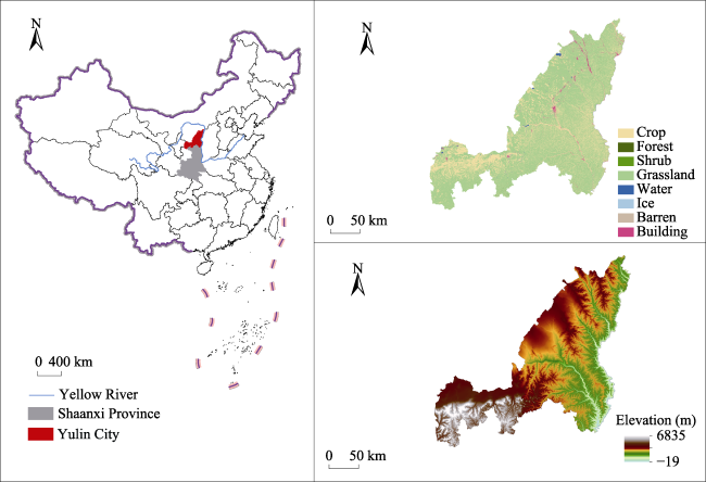
Figure 1 Location of study area

2.2 Data sources

This study utilized 2000-2018 satellite imagery, socioeconomic, and climate and environmental data. Satellite data at 30 m resolution were from GEE. Socioeconomic data included land use/land cover change at 30 m resolution, population density, and GDP raster at 1 km resolution, all from the Resources and Environmental Sciences Data Center. Climate and environmental data were precipitation (PRE, 30 m), temperature (TEM, 1 km), digital elevation model (DEM, 12.5 m), and aerosol optical depth (AOD, 30 m) from the Data Center and GEE (Table 1). For accuracy assessment, less cloudy Landsat images (July-September) were selected and de- clouded. As RSEI targets terrestrial ecosystems, large water bodies were masked (Xu, 2005).
Table 1 Interaction detection data
Data type Data name Resolution Data sources
Data base Landsat 5/7/8 30 m GEE (https://earthengine.google.com/)
LUCC 30 m Resources and Environmental Sciences and Data Center, Chinese Academy of Sciences (https://www.resdc.com/)
Socioeconomic data POP 1000 m Resources and Environmental Sciences and Data Center, Chinese Academy of Sciences (https://www.resdc.com/)
GDP 1000 m Resources and Environmental Sciences and Data Center, Chinese Academy of Sciences (https://www.resdc.com/)
Climate and environmental data PRE 30 m Resources and Environmental Sciences and Data Center, Chinese Academy of Sciences (https://www.resdc.com/)
TEM 1000 m Resources and Environmental Sciences and Data Center, Chinese Academy of Sciences (https://www.resdc.com/)
DEM 12.5 m Resources and Environmental Sciences and Data Center, Chinese Academy of Sciences (https://www.resdc.com/)
AOD 30 m GEE (https://earthengine.google.com/)

Note: GEE: Google Earth Engine; POP: population density data; GDP: gross domestic product; PRE: precipitation; TEM: air temperature; DEM: digital elevation model; AOD: aerosol optical depth.

2.3 Research methods

We developed a new MRSEI model incorporating FVC, EVI, LST, WET, and NDBSI within the original RSEI framework (Figure 2). MRSEI can overcome the limitation of NDVI being lowered by urban asphalt. NDVI was replaced with EVI and FVC to better characterize urban greenery. EVI complements FVC in sparse vegetation; together, they capitalize on EVI’s macro-scale assessment and offset FVC’s weakness in micro-scale investigation. Spatial autocorrelation analysis was used to examine spatiotemporal MRSEI changes and Yulin’s ecological environment. Geographic detectors were used to quantify the influence of socioeconomic, climate, and environmental factors on Yulin’s ecology using MRSEI.
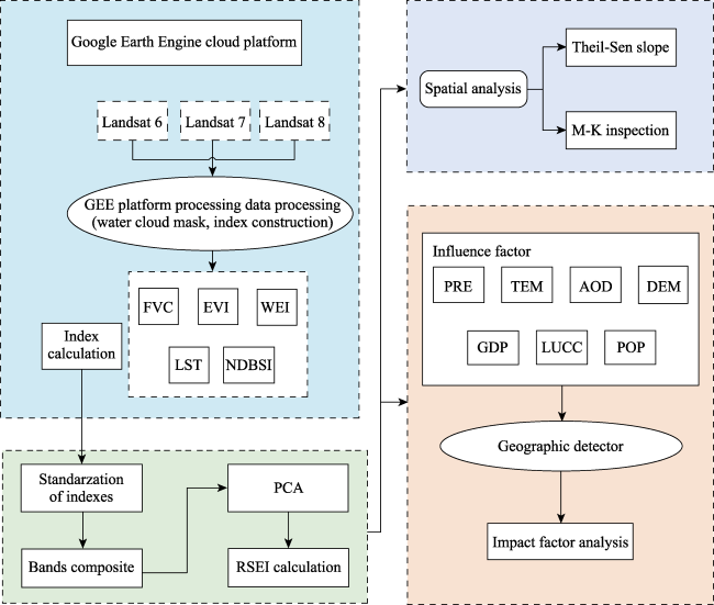
Figure 2 Methodological framework applied in this study

2.3.1 Construction of indicators

The MRSEI model integrates five indices: FVC, EVI, LST, WET, and NDBSI. PCA is employed to calculate the MRSEI. The study constructed index P, expressed as shown in Eq. (1):
$\begin{matrix} P=f\left( FVC,EVI,WET,LST,NDBSI \right) \\\end{matrix}$

2.3.2 Vegetation coverage

Research on vegetation coverage is currently extensive (Tucker, 1979; Hansen et al., 2000). The mainstream method (He et al., 2023) uses a pixel binary model to calculate the FVC in a study area, as expressed in Eq. (2):
$\begin{matrix} FVC=\frac{NDVI-NDV{{I}_{s}}}{NDV{{I}_{v}}-NDV{{I}_{s}}} \\\end{matrix}$
Where $~NDV{{I}_{v~}}$ represents is the NDVI value of the pure vegetation coverage pixels and $NDV{{I}_{s}}$ represents the NDVI values of bare soil pixels. The NDVI values of 5% and 95% are taken as confidence intervals; these were obtained within the confidence intervals NDVImin and NDVImax based on the FVC of the study area.

2.3.3 Enhanced Vegetation Indices

Compared to NDVI, EVI has advantages in reducing the impact of the background and atmosphere and can effectively eliminate the saturation problem in terms of the index. Currently, EVI is widely used in vegetation research with remarkable effects (Huete et al., 2002). The calculation for EVI is shown in Eq. (3):
$\begin{matrix} EVI=2.5\times \frac{{{\rho }_{nir}}-{{\rho }_{red}}}{{{\rho }_{nir}}+6{{\rho }_{red}}-7.5{{\rho }_{blue}}+1} \\\end{matrix}$
Where ${{\rho }_{nir}}$, ${{\rho }_{red}}$, and $~{{\rho }_{blue}}~$ represent the reflectance of the near-infrared band, red band, and blue band after atmospheric correction, respectively.

2.3.4 Humidity

The humidity index is the humidity component (WET) obtained according to the tasselled cap transformation and is calculated as shown in Eqs. (4)-(6)(Hu and Xu, 2018):
$\begin{align} & WET\left( 5 \right)=0.0325\times {{\rho }_{b}}+0.2021\times {{\rho }_{g}}+0.3012\times {{\rho }_{r}}+ \\ & 0.1594\times {{\rho }_{nir}}-0.6806\times SWI{{R}_{1}}-0.6109\times SWI{{R}_{2}} \\ \end{align}$
$\begin{matrix} WET\left( 7 \right)=0.2626\times {{\rho }_{b}}+0.2141\times {{\rho }_{g}}+0.0926\times {{\rho }_{r}}+ \\ 0.0656\times {{\rho }_{nir}}-0.7629\times SWI{{R}_{1}}-0.5388\times SWI{{R}_{2}} \\\end{matrix}$
$\begin{matrix} WET\left( 8 \right)=0.1509\times {{\rho }_{b}}+0.1973\times {{\rho }_{g}}+0.3279\times {{\rho }_{r}}+ \\ 0.3406\times {{\rho }_{nir}}-0.7112\times SWI{{R}_{1}}-0.4572\times SWI{{R}_{2}} \\\end{matrix}$
Where ${{\rho }_{b}}$,${{\rho }_{g}}$,${{\rho }_{r}}$,${{\rho }_{nir}}$ represent the reflectivity of bands blue, green, red and near infrared, respectively; $SWI{{R}_{1}}$ and $SWI{{R}_{2}}~$ represent the reflectivity of bands 1, 2, 3, 4, 5 and 7 of the Landsat 7 Enhanced Thematic Mapper (ETM+) and the reflectivity of bands 2, 3, 4, 5, 6, and 7 of the Landsat 8 Operational Land Imager (OLI)/Thermal Infrared Sensor (TIRS) respectively; WET (5) represents the humidity component of Landsat 5/TM; WET (7) represents the humidity component of Landsat 7 ETM+ imagery; and WET (8) represents the humidity component of Landsat 8 OLI/TIRS imagery.

2.3.5 Land surface temperature

The heat index is based on the LST and is calculated using Eqs. (7) and (8) (Chander et al., 2009):
$\begin{matrix} {{L}_{\lambda }}=gain\times DN+bias \\\end{matrix}$
$\begin{matrix} T=\frac{{{K}_{2}}}{\text{In}\left( \frac{{{K}_{1}}}{{{L}_{\lambda }}}+1 \right)} \\\end{matrix}$
where, ${{L}_{\lambda }}~$ is the radiation value of TM and OLI thermal infrared 6-band and 10-band pixels at the sensor; DN is the pixel grey value, and gain and bias are the gain value and bias value of the corresponding band, respectively; T represents the temperature reflected by the sensor; K1 and K2 are the calibration parameters, respectively: K1=606.09 W m–2 sr–1 μm–1, and K2 = 1282.71 K. Subsequently, an emissivity correction was performed on T, and the surface temperature, LST, was obtained as shown in Eq. (9):
$\begin{matrix} LST=\frac{T}{1+\left( \frac{\lambda T}{\rho } \right)\times \text{In}\varepsilon } \\\end{matrix}$
where λ is the central wavelength of TM and OLI thermal infrared bands 6 and 10; ρ=1.438 ×10⁻² mK; and ε is the surface emissivity, obtained according to the algorithm proposed by Nichol (Nichol, 2005).

2.3.6 Dryness

The dryness index (NDBSI) is composed of the bare soil index (SI) and building index (IBI) and is calculated using Eqs. (10)-(12) (Cristóbal et al., 2018):
$\begin{matrix} NDBSI=\frac{SI+IBI}{2} \\\end{matrix}$
$\begin{matrix} SI=\frac{\left( {{\rho }_{swir1}}+{{\rho }_{red}} \right)-\left( {{\rho }_{blue}}-{{\rho }_{nir}} \right)}{\left( {{\rho }_{swir1}}+{{\rho }_{red}} \right)+\left( {{\rho }_{blue}}+{{\rho }_{nir}} \right)} \\\end{matrix}$
and
$\begin{matrix} IBI=\frac{2\times \frac{{{\rho }_{swir2}}}{{{\rho }_{swir1}}+{{\rho }_{nir}}}-\left( \frac{{{\rho }_{nir}}}{{{\rho }_{red}}+{{\rho }_{nir}}}~+~\frac{{{\rho }_{green}}}{{{\rho }_{swir1}}+{{\rho }_{green}}} \right)}{2\times \frac{{{\rho }_{swir2}}}{{{\rho }_{swir1}}+{{\rho }_{nir}}}+\left( \frac{{{\rho }_{nir}}}{{{\rho }_{red}}+{{\rho }_{nir}}}~+~\frac{{{\rho }_{green}}}{{{\rho }_{swir1}}+{{\rho }_{green}}} \right)} \\\end{matrix}$
where, ${{\rho }_{swir1}}$,${{\rho }_{swir2}}$,${{\rho }_{red}},{{\rho }_{green}}$,${{\rho }_{blue}}$,${{\rho }_{nir}}$are the reflectivities of the short infrared 1, short infrared 2, red, green, blue, and near infrared bands, respectively.

2.4 Normalization Processing

The five selected ecological indicators were normalized to the [0,1] range using min-max scaling, with the transformation formula defined as:
$\begin{matrix} {{A}_{i}}=\frac{{{B}_{i}}-{{B}_{\min }}}{{{B}_{\max }}-{{B}_{\min }}} \\\end{matrix}$
Where ${{A}_{i}}$ is the standardised processing value of the i-th index; ${{B}_{i}}$ is the i-th original indicator value; Bmax is the i-th maximum indicator value; and Bmin is the i-th minimum indicator value.

2.5 Principal component analysis

After normalizing the indices, the RSEI values were obtained using PCA, which is a widely used statistical method for data analysis (Bro and Smilde, 2014) that can transform variables that may be correlated into linearly uncorrelated variables through orthogonality, which has the advantages of objectivity and reduced errors in statistical data (Gower, 1966). The concrete steps were: 1) Standardization of index data, 2) Determination of the correlation between indicators, 3) Determine all the calculated principal components, and 4) Determination of the weight of the principal components. The calculation formula is shown in Eq. (14):
$\begin{matrix} P=\underset{i=1}{\overset{k}{\mathop \sum }}\,{{e}_{i}}\times p{{c}_{i}} \\\end{matrix}$
where P is the ecological comprehensive index,${{e}_{i}}$(i =1, 2, $\cdots $, k) is the variance contribution rate of each principal component, k is the number of selected principal components, and $p{{c}_{i~}}$ is the corresponding i-th principal component.

2.6 Moran’s I Index

The Moran’s I index is a vital spatial statistical tool that detects spatial autocorrelation to uncover global clustering patterns, reflects regional-scale spatial associations, and evaluates heterogeneity across the study area (Anselin, 1995; Getis and Ord, 2008).

2.7 Geographical Detector Model

The recently proposed geographic detector model identifies driving factors through independent linear functions, effectively revealing hidden mechanisms in complex systems (Wang et al., 2017; Zhu et al., 2020; Nie et al., 2021). Using precipitation, temperature, air quality (AOD), elevation, GDP, land use, and population density (POP) as independent variables, we apply the geographic detector model to analyse drivers of ecological environment quality change in Yulin City.

2.8 Construction of MRSEI model

We have created a new model, MRSEI, to evaluate urban ecology. To do this, we used Landsat satellite images to calculate five indicators (FVC, EVI, WET, NDBSI, and LST) on the GEE platform. We then normalized these indicators and used principal component analysis to calculate the MRSEI values.

3 Analysis of results

3.1 MRSEI model validation

3.1.1 Data correlation analysis

In this study, the average values of FVC, EVI, LST, WET, NDBSI, and MRSEI for Yulin City were calculated over a continuous period of 21 years utilizing the Google Earth Engine platform. Following this, a randomized selection of 40000 sample points was performed to conduct a correlation analysis between each individual factor and the MRSEI values. The primary objective of this analysis was to investigate the connections between different factors and MRSEI.
As illustrated in Figure 3, all factors within the MRSEI demonstrated robust linear relationships. FVC exhibited the highest Pearson correlation coefficient of 0.993 with MRSEI, followed by EVI and WET with correlation coefficients of 0.964 and 0.625, respectively, the average correlation was 0.840. NDBSI and LST showed negative correlation coefficients of -0.840 and -0.779 with MRSEI, respectively, both of which passed significance testing. To compare with the traditional RSEI index, we conducted a Pearson correlation test between NDVI and RSEI, resulting in a correlation coefficient of 0.895, which is lower than the coefficients of 0.993 for FVC and 0.964 for EVI. This suggests that FVC and EVI exhibit stronger linear relationships when compared with NDVI, rendering them more suitable replacements.
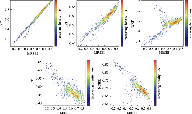
Figure 3 The five indicators of MRSEI point density

3.1.2 MRSEI and RSEI indicators comparison

To validate MRSEI, we compared its main components to traditional RSEI for 2018, an ecologically improved year (Table 2). MRSEI’s PC1 was 90.23%, 12.88 percentage points higher than traditional RSEI’s 77.35%, improving calculation accuracy.
Table 2 Principal component analysis results of MRSEI and RSEI indicators in 2018
Indicators PCA NDVI FVC EVI WET NDBSI LST Percent eigenvalue


MRSEI

PC1 - 0.870 0.347 0.241 -0.271 -0.242 90.23%
PC2 - 0.237 0.225 -0.214 -0.01 0.921
PC3 - -0.334 0.068 0.665 -0.628 0.218
PC4 - -0.262 0.778 -0.427 -0.306 -0.224

RSEI
PC1 0.623 - - 0.398 -0.514 -0.434 77.35%
PC2 0.368 - - 0.080 -0.246 0.893
PC3 -0.468 - - 0.876 -0.012 0.117
PC4 -0.507 - - -0.260 -0.821 0.006

Note: “-”: No corresponding indicator.

The positive/negative correlations between MRSEI metrics agreed with RSEI. FVC, EVI, and WET positively correlated with PC1, promoting ecological quality, while LST and NDBSI negatively correlated, indicating inhibitory effects. For MRSEI, PC1 absolute values ranked: FVC>EVI> NDBSI>LST>WET; for RSEI: NDVI>NDBSI>LST>WET. The order aligned with RSEI and ecological conditions. In summary, MRSEI improves accuracy, and its five indices better reflect urban ecology.

3.1.3 RSEI and MRSEI Model comparison

A comparison plot between MRSEI and RSEI models was generated as shown below:
Figure 4 shows similar trends for MRSEI and RSEI, but MRSEI values were higher than RSEI, which aligns with the low NDVI values in urban ecology, causing spatial distribution differences. To elucidate the differences between the two methods, we compared RSEI and MRSEI across four land cover types, namely road, cropland, village, wasteland, identified from satellite images.
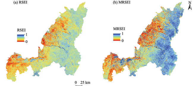
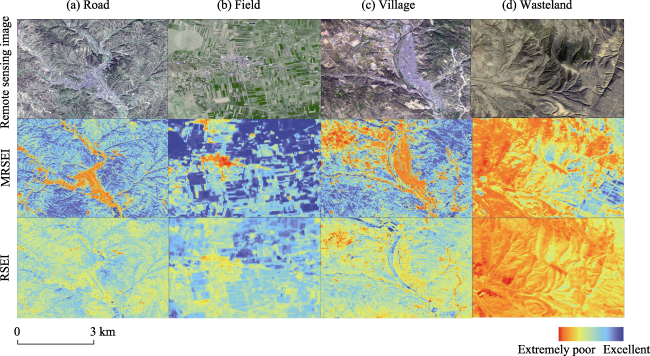
Figure 4 Comparation between MRSEI and RSEI
As shown in Figure 5, MRSEI exhibited more intricate details in contrast to the conventional RSEI. In the road segment of Figure 5a, MRSEI significantly improved the image texture compared with RSEI. Figure 5b portrays an ecologically healthy field, within which satellite imagery highlights a wasteland patch more distinctly identified by MRSEI than RSEI. Figure 5c illustrates a village encompassing developed land, with its boundaries appearing crisper in MRSEI compared with RSEI. Figure 5d displays a wasteland region characterized as ecologically less favourable, while satellite imagery reveals a forest in the southeast direction that is more clearly distinguishable through MRSEI. Overall, in comparison to RSEI, MRSEI provided enhanced recognition of regional details, aligning ecological quality representation more closely with actual ground conditions.
Figure 5 Comparation of local details between MRSEI and RSEI

3.2 Principal component analysis

We selected the first principal component of five Landsat indicators from 2000, 2005, 2010, 2015, and 2018. These were calculated on GEE together with MRSEI (Table 3).
Table 3 Eigenvalues of each principal component and their contribution rates
Year MRSEI First principal component (PC1) PC1 Contribution rate (%)
FVC EVI WET LST NDBSI
2000 0.439 0.9045 0.2116 0.2269 0.2006 0.2133 83.3647
2005 0.459 0.8825 0.2392 0.2744 0.2055 0.2154 84.9005
2010 0.489 0.9052 0.0562 0.2354 0.1715 0.3042 91.8367
2015 0.488 0.8211 0.2309 0.2524 0.3632 0.2771 86.3276
2018 0.518 0.8703 0.4471 0.2414 0.2423 0.2711 90.2383

Note: FVC: fractional vegetation coverage; EVI: enhanced vegetation index; WET: wet index; LST: land surface temperature; NDBSI: normalized difference building-soil index; PC1: first principal component.

In Table 3, PC1 contributed 83.36% to 91.84% of MRSEI variation in Yulin City from 2000 to 2018. PC1 loads positively on FVC, EVI, and WET and negatively on LST and NDBSI, reflecting that more vegetation and humidity indicate better Yulin ecology. Higher LST and dryness reflecting worse ecology aligns with the real ecological influence of these indicators. PC1 well represents the five indicator components; thus, using it to calculate MRSEI enhances accuracy.

3.3 Temporal variation of Yulin’s ecological environment quality

3.3.1 Dynamic changes in ecological environment quality

To depict recent changes in Yulin City’s ecological environment more clearly, MRSEI values were categorized into five grades: extremely poor (0-0.2), poor (0.2-0.4), medium (0.4-0.6), good (0.6-0.8), and excellent (0.8-1). Table 4 lists the MRSEI value distribution in Yulin City.
Table 4 Change in area ratios for ecological grades
Grade Area ratio (%) 2000-2018
2000 2005 2010 2015 2018
Extremely poor 17.99 13.06 12.73 10.73 12.59 -5.4
Poor 36.88 25.09 22.25 24.1 19.02 -17.86
Moderate 28.89 35.91 31.27 28.53 25.55 -3.34
Good 12.37 19.88 25.1 25.04 33.02 20.65
Excellent 3.87 6.06 8.65 11.6 9.82 5.95
The average MRSEI in Yulin City increased from 0.479 to a peak of 0.518 between 2000 and 2018, indicating improved ecological quality. As Table 4 shows, Yulin has a small proportion of Good/Excellent grades and a poor ecological base. The combined Poor/Fair area decreased 23.26% while Good/Excellent area increased 26.60%, reflecting Yulin’s overall upward ecological trend. However, a slight decline occurred from 2015-2018, with a 1.78% Excellent grade reduction. In summary, while improving from 2000 to 2018, Yulin’s ecology declined slightly after 2015, warranting attention.

3.3.2 Ecological environment quality grade transfer analysis

To further monitor ecological quality grade changes, the classified MRSEI results for each period were overlaid in ArcGIS, and a transfer matrix extracted the grade transition map (Figure 6).
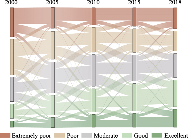
Figure 6 MRSEI level change statistics
The transition matrix clearly depicted the direction and magnitude of ecological grade changes in Yulin City from 2000 to 2018. Integrated with statistical data, results showed the ecological environment underwent significant transformations: 1) Transitions were mainly from Extremely poor to Moderate and Moderate to Good. The largest Extremely poor to Moderate shift occurred in 2000-2005 (6586.5951 km2). The maximum Moderate to Good change was in 2010-2015 (5146.2621 km2). 2) The largest Excellent to Good transition was 561.8205 km2 (2000-2005). The maximum Good to Excellent was 3050.5554 km2 (2015-2018). 3) The greatest Good to Moderate change was 2977.7031 km2 (2010-2015). 4) Aside from Moderate to Good, the largest transition from Moderate was to Extremely poor (3390.7167 km2 in 2010-2015). 5) Aside from Extremely poor, the maximum Moderate to Poor conversion was 2821.6323 km2 (2015-2018). 6) Aside from Extremely poor, Poor to other grade transitions were small, with the minimum being Poor to Excellent (52.2162 km2 in 2010-2015).

3.4 Spatial variation of Yulin’s ecological quality

3.4.1 Spatial distribution analysis

Spatially, following previous classification standards, we created a five-year map depicting changes in the ecological environment quality of Yulin City. The results are presented in Figure 7.
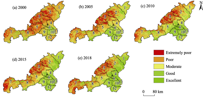
Figure 7 Changes in the ecological quality of Yulin City

Note: 1: Fugu County; 2: Shenmu City; 3: Yuyang District; 4: Jia County; 5: Hengshan District; 6: Mizhi County; 7: Dingbian County; 8: Jingbian County; 9: Zizhou County; 10: Suide County; 11: Wubao County; 12: Qingjian County.

Spatially, Yulin’s ecology follows a “good southeast, poor northwest” pattern. Good ecological areas (0.6-1 MRSEI) concentrate in the southeast counties and parts of northeast Yulin, while poor areas (0-0.4 MRSEI) concentrate in west Yulin and northern Yuyang. Yulin slopes west-to-east with lower southeast terrain near Qingjian suitable for vegetation versus higher west/north areas in Dingbian/Yuyang with sparser vegetation and fragile ecology. In summary, Yulin has predominantly Extremely poor/Moderate ecology, with Poor/Extremely poor levels in high-altitude, arid areas, and Good/Excellent levels in lowlands.

3.4.2 Spatial variation analysis

To better visualize Yulin’s ecological changes, the ArcGIS raster calculator subtracted imagery rasters, with results classified into five equal intervals: Obvious Deterioration, Slight Deterioration, No Change, Slight Improvement, and Obvious Improvement (Figure 8).
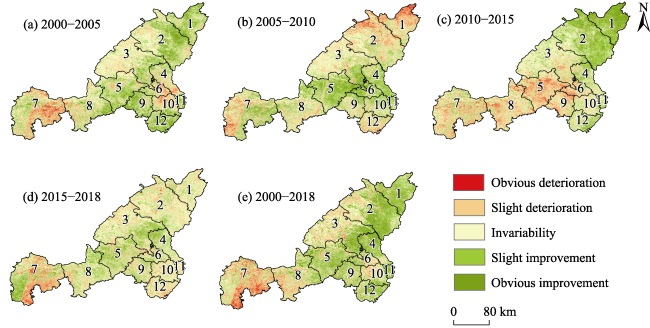
Figure 8 Distribution of eco-environmental quality change categories in Yulin City

Note: 1: Fugu County; 2: Shenmu City; 3: Yuyang District; 4: Jia County; 5: Hengshan District; 6: Mizhi County; 7: Dingbian County; 8: Jingbian County; 9: Zizhou County; 10: Suide County; 11: Wubao County; 12: Qingjian County.

The ecological quality in Yulin City from 2000 to 2018 exhibited slight to obvious improvement, primarily in the eastern counties of Qingjian, Wubao, Jia, and Fugu, alongside the central Hengshan District and Zizhou County. Obvious deterioration occurred mainly in high-altitude, desertified areas of western Dingbian County and northern Yuyang District. From 2005 to 2010, ecological quality was largely unchanged. Deterioration was most extensive from 2010 to 2015, concentrated in Hengshan District, Jingbian County, and Zizhou County. After 2015, the greatest ecological improvements emerged in previously deteriorated areas, likely reflecting Yulin’s ecological protection policies and suggesting successful governance. Overall, ecological governance in Yulin City has substantially increased areas of improvement, with lingering deterioration mostly constrained to western areas, enhancing ecological quality.

3.4.3 Spatial autocorrelation analysis

To analyse the spatial heterogeneity of MRSEI in Yulin City, the Moran’s I index was used to assess spatial autocorrelation. The calculated MRSEI raster was converted to vector point data for implementing spatial autocorrelation analysis in ArcGIS. The analysis revealed spatial clustering patterns of MRSEI in Yulin City, as illustrated by the Local Indicator of Spatial Association (LISA) cluster map shown in Figure 9.
Figure 9 LISA cluster diagram of MRSEI index

Note: 1: Fugu County; 2: Shenmu City; 3: Yuyang District; 4: Jia County; 5: Hengshan District; 6: Mizhi County; 7: Dingbian County; 8: Jingbian County; 9: Zizhou County; 10: Suide County; 11: Wubao County; 12: Qingjian County.

The Moran’s I and z-values for the five-time periods in Yulin City were statistically significant, indicating positive spatial autocorrelation of the MRSEI index. Spatially, Yulin City showed heterogeneous patterns of ecological quality. High-high clusters were primarily situated in the low-altitude eastern counties, while low-low clusters predominated in the high-altitude, desertified western and northern districts. Areas of non-significance gradually declined, mainly in the central counties. Before 2010, the distribution of ecological quality was relatively stable. After 2010, the coverage of high-high
clusters expanded, but internal heterogeneity significantly increased, suggesting ecological improvement coupled with decreasing stability from 2010 to 2018. Specifically, northeastern Fugu County and Shenmu City transitioned from non-significant to high-high clusters from 2000 to 2018, implying ecological improvement but poor resilience to disturbances.

3.5 Analysis of influencing factors

3.5.1 Factor exploration

To explore the factors affecting the MRSEI index of Yulin City, a geographical detector was used for factor analysis. Seven environmental indicators, Elevation, PRE, GDP, POP, AOD, TEM, and LUCC, for Yulin City in 2018 were selected as independent variables of the geographical detector, and the MRSEI value of Yulin City in 2020 was selected as the dependent variable. ArcGIS software was used to create a fishing net tool. Subsequently, the created surface elements were converted into points, the established point elements were imported into Excel, and abnormal points were removed. A total of 4652 eliminated elements were imported into the geographical detector model. The results in Table 5 indicate that all factors passed the significance test (P<0.01). However, these factors varied in their explanatory power for the ecological environment. The explanatory power ranked as follows: PRE (0.259)>Elevation (0.158)>LUCC (0.139)>TEM (0.115)>POP (0.055)>GDP (0.053)>AOD (0.036). Among these factors, PRE was the most significant factor influencing the ecology of Yulin City. Elevation, TEM, and LUCC, with P-values greater than 0.1, play a secondary role in impacting the ecology of Yulin City. Additionally, AOD has minimal ecological impact on Yulin City, and this study suggests that it is not a suitable indicator for calculation.
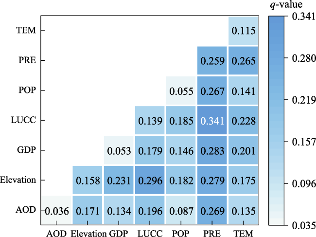
Table 5 q-values for factor exploration
Factor TEM PRE Elevation AOD POP LUCC GDP
q 0.115 0.259 0.158 0.036 0.055 0.139 0.053
P <0.001 <0.001 <0.001 <0.001 <0.001 <0.001 <0.001

Note: TEM: air temperature; PRE: precipitation; AOD: aerosol optical depth; POP: population density data; LUCC: land use and cover change; GDP: gross domestic product.

3.5.2 Interactive exploration

Using the interaction detector to investigate factor interactions, the combined explanatory power of two interacting factors surpasses that of each individual factor, suggesting that inter-factor interactions have a more substantial influence on Yulin’s ecology. The most significant interaction was observed between PRE and LUCC, with a two-factor interaction q value of 0.341 (Figure 10). Conversely, the weakest explanatory power was in the interaction between POP and AOD, possibly attributed to the geomorphological features of Yulin City, leading to uneven population distribution and insufficient explanatory capability when these two factors interacted. Combinations involving PRE and most other factors yield high q-values, with the lowest being the combination of PRE and POP, which reached 0.267. This suggests the paramount importance of PRE in influencing the ecology of Yulin City.
Figure 10 Interactive exploration results

Note: LUCC: land use and cover change; TEM: air temperature; PRE: precipitation; POP: population density data; GDP: gross domestic product; AOD: aerosol optical depth.

3.5.3 Risk exploration

Using the risk detector, we determined the range of MRSEI values among the factors (Figure 11). Regarding socioeconomic data, as GDP increased, the MRSEI value initially decreased, then gradually increased, reaching a peak of 5091×104 yuan in 1975. Population density (POP) exhibited a steady increase, peaking at 23400 persons km-2, before declining.
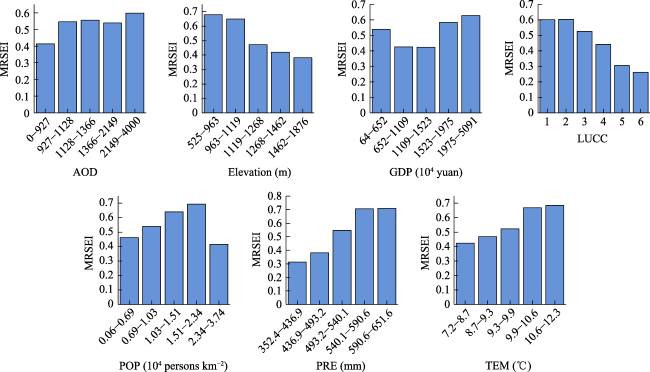
Figure 11 Statistical results for MRSEI at various levels of influencing factors

Note: LUCC: land use and cover change; 1: Farmland; 2: Forest; 3: Grassland; 4: Water; 5: Urban, rural, industrial, mining, and residential lands; 6: Wasteland; TEM: air temperature; PRE: precipitation; POP: population density data; GDP: gross domestic product; AOD: aerosol optical depth.

Concerning climate and environmental data, MRSEI demonstrated a declining trend with increasing Elevation, and the optimal range for Elevation was between 525 and 963 m. As the temperature increased, MRSEI exhibited a consistent upward trend, reaching a maximum temperature of 10.6-12.3 ℃. With rising precipitation, the MRSEI index gradually increased and stabilized, peaking at 590.6- 651.6 mm of precipitation. Regarding land use, the MRSEI index varied based on land use type. The MRSEI value was highest for Farmland and lowest for Wasteland, consistent with the real-world situation.

3.5.4 Ecological exploration

We employed the ecological detector to compare the spatial distribution differences of MRSEI between the two factors. Table 6 reveals no significant differences in the MRSEI index between AOD and GDP data, and GDP and POP. However, the combinations of other factors exhibit substantial differences in MRSEI values.
Table 6 Statistical significance of ecological monitoring factors
Factor AOD Elevation GDP LUCC POP PRE TEM
AOD
Elevation Y
GDP N Y
LUCC Y Y Y
POP Y Y N Y
PRE Y Y Y Y Y
TEM Y Y Y Y Y Y

Note: AOD: aerosol optical depth; GDP: gross domestic product; LUCC: land use and cover change; POP: population density data; PRE: precipitation; TEM: air temperature.

4 Discussion

4.1 Rationality of MRSEI

RSEI is widely used in urban- and watershed-scale regional ecological assessment research. However, in geographic landscape area research, RSEI is not as effective. To promote the accuracy of the RSEI calculations, the study proposes a new computational method MRSEI; the evaluation index of NDVI was replaced with FVC and EVI, and a new RSEI formula was created (Eq. 1). MRSEI exhibits advantages over traditional RSEI in vegetation monitoring. Our study shows significant correlations between the five indicators and MRSEI. With respect to the contribution rate of the primary principal component, MRSEI exhibited a 12.88% improvement over RSEI, facilitating more precise calculations. Compared with real imagery, MRSEI demonstrated enhanced capabilities in identifying roads, buildings, and vegetation, rendering it suitable for assessing regional ecological quality.

4.2 MRSEI applicability

Utilizing the MRSEI model, we conducted a spatiotemporal analysis of Yulin City’s ecological quality. The findings indicate that MRSEI offers distinct advantages for urban ecological assessment. In comparison to the traditional RSEI, MRSEI provides a more precise reflection of urban ecological quality. To gain deeper insights into MRSEI’s applicability in a river basin context, we selected the Yanhe River Basin as our experimental subject. The outcomes are depicted in Figure 12.
Figure 12 Comparation between MRSEI and RSEI in Yanhe River Basin
Figure 12 reveals that at the basin level, MRSEI and RSEI exhibit spatial consistency, with the southern region displaying superior ecology while the northern and eastern regions exhibit weaker ecology. However, there is localized differentiation in specific details. To achieve this, the study integrated regional images and compared them with the calculated result map, as illustrated in Figure 13.
Figure 13 Comparison of Local Details in Yanhe River Basin
Compared with the actual landscape, MRSEI offers distinct advantages in depicting the village, road, and wasteland within the watershed. Regarding villages, MRSEI, when compared with RSEI, excels in distinguishing landforms like villages from the surrounding vegetation-covered areas, with a higher degree of clarity in differentiation. Traditional RSEI tends to link roads with unused and ecologically poor land, making accurate identification challenging. In contrast, MRSEI can distinguish roads from other landforms with greater accuracy. When identifying unused land, MRSEI can accurately determine and calculate the vegetation cover area in extensive unused land, leading to more precise calculation results.
In summary, MRSEI is applicable to ecological assessments in watershed areas. For instance, in extensive unused land, only a small portion may have better ecological characteristics. However, traditional RSEI may fail to identify this, resulting in calculation bias. Additionally, traditional RSEI may not accurately identify other ecologically poor areas like roads. In terms of vegetation, MRSEI leverages the complementary attributes of FVC and EVI in areas with high and low vegetation cover. This approach enhances the depiction of regional vegetation growth status and improves calculation accuracy. MRSEI exhibits broad applicability, suitable not only for urban ecological assessments but also for watershed-level ecological assessments.

4.3 Analysis of ecological factors in Yulin City 4.3.1 Impact factor analysis

Utilizing the geographical detector model, we conducted an analysis of the influencing factors in Yulin City during 2018. Our findings highlight precipitation as the primary factor, with a q-value of 0.259. Precipitation impacts vegetation growth in Yulin City, triggering changes in land use and other data that result in environmental shifts. Furthermore, national spatial planning and its related ecological conservation policies constitute an additional significant factor influencing regional ecological quality (Cao et al., 2009; Li et al., 2016; Kang et al., 2021). Upon examining Yulin’s recent environmental protection policies, we observed a simultaneous increase in MRSEI values following the implementation of each new policy. As an example, the initiation of the Grain for Green project in 2005 resulted in a 1.5% increase in MRSEI from 2005 to 2006. Furthermore, we integrated the environmental factor AOD into the geographical detector model for the first time. The resulting q value of 0.036 was the lowest among all factors, indicating limited explanatory capacity for variations in MRSEI. Thus, it might not be optimal to utilize it as a computational indicator (Wang et al., 2023).

4.3.2 MRSEI classification intervals

Based on risk detector calculations, the optimal MRSEI range was identified. Yulin City’s ecological quality thrives in conditions of high rainfall, elevated humidity, and favourable temperatures (Table 7). The ecological condition is at its best when the predominant land types are farmland and grassland. At lower altitudes, Elevation peaks between 525 and 926 m, which is more conducive to vegetation growth. Regarding human activities, Yulin’s MRSEI index aligns better with a high GDP and an appropriate population density. This correlation may be attributed to Yulin’s ecological and environmental protection policies, where higher GDP leads to increased government investment in ecology.
Table 7 Significance statistics of ecological detection factors
Driving factors MRSEI suitability MRSEI
TEM 10.6-12.3 (℃) 0.6-0.7
PRE 590.6-651.6 (mm) 0.6-0.7
Elevation 525-926 (m) 0.6-0.7
AOD 2149-4000 0.5-0.6
GDP 1975-5091 (104 yuan) 0.6-0.7
POP 1.51-2.34 (104 persons km-2) 0.6-0.7
LUCC Crop 0.5-0.6

4.4 Future research and outlook

This study put forward a novel calculation method to calculate the quality of the regional ecological environment and was verified by Yulin City. The results showed that the ecological index calculated by our calculation method was more realistic. However, our study has some limitations. First, we used an improved eco-environmental quality assessment method that focused on greenness, humidity, heat, and dryness. However, ecosystems are complex and diverse and include both natural and socioeconomic development factors. Only the ecological index was used to construct the RSEI. Future studies should include additional indicators. In addition, the weight of each indicator should be analysed to create a more robust indicator system. Second, as artificial intelligence grows in popularity, it is increasingly being used in remote sensing ecological monitoring and analysis (Zhang et al., 2016; Singh et al., 2018; Kroupi et al., 2019). Therefore, the combination of artificial intelligence and RSEI may be used to evaluate regional ecological environment quality more accurately. For example, future research should explore the construction of scientific assessment systems or ecological prediction models by using neural networks.

5 Conclusions

(1) The MRSEI model offers a more precise assessment of regional ecological quality compared with the RSEI model. In terms of data correlation, the Pearson correlation coefficients between FVC and EVI for MRSEI were 0.993 and 0.964, respectively, higher than those of NDVI and 0.895 for RSEI. This indicates a stronger correlation between FVC and EVI. The average correlation between the five indicators and MRSEI was 0.840. PC1’s contribution was 12.88% greater than that of RSEI, reflecting regional ecology more accurately. MRSEI also improved its capability in identifying roads, villages, and unused land compared with satellite images. Additionally, it demonstrated enhanced sensitivity to vegetation, providing a more accurate representation of the real situation. Consequently, MRSEI more accurately reflected the status of regional ecological quality.
(2) MRSEI calculation showed Yulin City’s ecological quality trending upward, peaking at 0.518 in 2018. The 21-year average of 0.481 indicated a relatively poor foundation. Approximately 38.81% of the area improved ecologically, while 10.15% significantly decreased. Spatially, Yulin City’s ecology exhibits a “southeast superior, northwest inferior” pattern. Higher quality areas were concentrated in the southeast Mizhi, Suide, Zizhou counties and northeast Jia County, Shenmu City, eastern Fugu County. Poorer areas were in western and northern Yulin, Dingbian County, and Yuyang District.
(3) Yulin City exhibits relatively stable ecological quality. The regions displaying high-high clusters were primarily situated in the low-altitude eastern and central areas, indicating better ecological quality. Conversely, the western high-altitude and northern desert areas of Yulin City predominantly exhibited low-low clusters, signifying poorer ecological quality. Post-2010, the eastern high-high cluster area had notably expanded, reflecting improved ecological quality. However, the high-low cluster area also increased, indicating insufficient ecological stability and susceptibility to natural and human influences.
(4) The MRSEI model was effective not only in assessing urban ecological quality but also basin ecological quality assessment, making it suitable for large-scale applications.
[1]
Alonzo M, Bookhagen B, Roberts D A. 2014. Urban tree species mapping using hyperspectral and lidar data fusion. Remote Sensing of Environment, 148: 70-83.

[2]
Anselin L. 1995. Local indicators of spatial association-LISA. Geographical Analysis, 27(2): 93-115.

[3]
Ariken M, Zhang F, Liu K, et al. 2020. Coupling coordination analysis of urbanization and eco-environment in Yanqi Basin based on multi-source remote sensing data. Ecological Indicators, 114(16): 106331. DOI: 10.1016/j.ecolind.2020.106331.

[4]
Bro R, Smilde A.K. 2014. Principal component analysis. Analytical methods, 6(9): 2812-2831.

[5]
Cao S X, Li C, Yu X X. 2009. Impact of China’s grain for green project on the landscape of vulnerable arid and semi-arid agricultural regions: A case study in Northern Shaanxi Province. Chinese Journal of Applied Ecology, 46(3): 536-543. (in Chinese)

[6]
Chander G, Markham B L, Helder D L. 2009. Summary of current radiometric calibration coefficients for Landsat MSS, TM, ETM+, and EO-1 ALI Sensors. Remote Sensing of Environment, 113(5): 893-903.

[7]
Chen L X, Zhu W Q, Zhou X J, et al. 2003. Characteristics of the heat island effect in Shanghai and its possible mechanism. Advances in Atmospheric Sciences, 20(6): 991-1001.

[8]
Cristóbal J, Jiménez-Muñoz J C, et al. 2018. An improved single-channel method to retrieve land surface temperature from the Landsat-8 thermal band. Remote Sensing, 10(3): 431. DOI: 10.3390/rs10030431.

[9]
Cumming G.S, Buerkert A, Hoffmann E M, et al. 2014. Implications of agricultural transitions and urbanization for ecosystem services. Nature, 515(7525): 50-57.

[10]
Getis A, Ord J K. 2008. The analysis of spatial association by use of distance statistics. Geographical Analysis, 24(3): 189-206.

[11]
Gower J C. 1966. Some distance properties of latent root and vector methods used in multivariate analysis. Biometrika, 53(3-4): 325-338.

[12]
Grimmond S U E. 2007. Urbanization and global environmental change: local effects of urban warming. The Geographical Journal, 173(1): 83-88.

[13]
Hansen M, DeFries R, Townshend J R, et al. 2000. Global land cover classification at 1km resolution using a decision tree classifier. International Journal of Remote Sensing, 21(6-7): 1331-1365.

[14]
He C Y, Gao B, Huang Q X, et al. 2017. Environmental degradation in the urban areas of China: Evidence from multi-source remote sensing data. Remote Sensing of Environment, 193(1): 65-75.

[15]
He C Y, Liu Z F, Tian J, et al. 2014. Urban expansion dynamics and natural habitat loss in China: a multiscale landscape perspective. Global Change Biology, 20(9): 2886-2902.

DOI PMID

[16]
He Z L, Yue T M, Chen Y L, et al. 2023. Analysis of spatial and temporal changes in vegetation cover and driving forces in the Yan River Basin, Loess Plateau. Remote Sensing, 15(17): 4240. DOI: 10.3390/rs15174240.

[17]
Hu X S, Xu H Q. 2018. A new remote sensing index for assessing the spatial heterogeneity in urban ecological quality: A case from Fuzhou City, China. Ecological Indicators, 89(8): 11-21.

[18]
Huete A, Didan K, Miura T, et al. 2002. Overview of the radiometric and biophysical performance of the MODIS vegetation indices. Remote Sensing of Environment, 83(1-2): 195-213.

[19]
Kang J M, Zhang X, Zhu X W, et al. 2021. Ecological security pattern: A new idea for balancing regional development and ecological protection. A case study of the Jiaodong Peninsula, China. Global Ecology and Conservation, 26(1): e01472. DOI: 10.1016/j.gecco.2021.e01472.

[20]
Kroupi E, Kesa M, Navarro Sánchez V D, et al. 2019. Deep convolutional neural networks for land-cover classification with sentinel-2 images. Journal of Applied Remote Sensing, 13(2): 024525. DOI: 10.1117/1.JRS.13.024525.

[21]
Li S, Wei L, Fu B J, et al. 2016. Vegetation changes in recent large-scale ecological restoration projects and subsequent impact on water resources in China’s Loess Plateau. Science of the Total Environment, 569: 1032-1039.

[22]
Liu L, Coops N C, Aven N W, et al. 2017. Mapping urban tree species using integrated airborne hyperspectral and lidar remote sensing data. Remote Sensing of Environment, 200: 170-182.

[23]
Martínez B, Camacho F, Verger A, et al. 2013. Intercomparison and quality assessment of MERIS, MODIS and SEVIRI FAPAR products over the Iberian Peninsula. International Journal of Applied Earth Observation and Geoinformation, 21(1): 463-476.

[24]
Nichol J. 2005. Remote sensing of urban heat islands by day and night. Photogrammetric Engineering & Remote Sensing, 71(5): 613-621.

[25]
Nie T, Dong G T, Jiang X H, et al. 2021. Spatio-temporal changes and driving forces of vegetation coverage on the Loess Plateau of Northern Shaanxi. Remote Sensing, 13(4): 613. DOI: 10.3390/rs13040613.

[26]
Petrou Z I, Manakos I, Stathaki T. 2015. Remote sensing for biodiversity monitoring: A review of methods for biodiversity indicator extraction and assessment of progress towards international targets. Biodiversity and Conservation, 24(10): 2333-2363.

[27]
Pettorelli N. 2013. The normalized difference vegetation index. OUP Oxford, USA: Google Books.

[28]
Rouse J W, Haas R H, Schell J A, et al. 1974. Monitoring vegetation systems in the great plains with ERTS. NASA Special Publication, 351(1): 309.

[29]
Singh A K, Ganapathysubramanian B, Sarkar S, et al. 2018. Deep learning for plant stress phenotyping: trends and future perspectives. Trends in Plant Science, 23(10): 883-898.

DOI PMID

[30]
Tan Y T, Xu H, Zhang X L. 2016. Sustainable urbanization in China: A comprehensive literature review. Cities, 55: 82-93.

[31]
Teng Y G, Wu J, Lu S J, et al. 2014. Soil and soil environmental quality monitoring in China: A review. Environment International, 69: 177-199.

DOI PMID

[32]
Tucker C J. 1979. Red and photographic infrared linear combinations for monitoring vegetation. Remote sensing of Environment, 8(2): 127-150.

[33]
Wang F G, Xu Y J. 2009. Comparison of remote sensing change detection techniques for assessing hurricane damage to forests. Environmental Monitoring and Assessment, 162(1-4): 311-326.

[34]
Wang J F, Xu C D. 2017. Geodetector: Principle and prospective. Acta Geographica Sinica, 72(1): 116-134. (in Chinese)

DOI

[35]
Wang X L, Zhang S R, Zhao X, et al. 2023. Exploring the relationship between the eco-environmental quality and urbanization by utilizing sentinel and Landsat data: A case study of the Yellow River Basin. Remote Sensing, 15(3): 743. DOI: 10.3390/rs15030743.

[36]
Wang Z C, He X H. 2021. Assessments of ecological quality in Jinjiang district of Chengdu City using the FVC and RSEI models. Journal of Ecology and Rural Environment, 37(4): 492-500. (in Chinese)

[37]
Wen X L, Ming Y L, Gao Y G, et al. 2019. Dynamic monitoring and analysis of ecological quality of Pingtan comprehensive experimental zone, a New Type of Sea Island City, Based on RSEI. Sustainability, 12(1): 21. DOI: 10.3390/su12010021.

[38]
Wu S P, Gao X, Lei J Q, et al. 2022. Ecological environment quality evaluation of the Sahel region in Africa based on remote sensing ecological index. Journal of Arid Land, 14(1): 14-33.

DOI

[39]
Xu H Q. 2005. A study on information extraction of water body with the modified normalized difference water index (MNDWI). Journal of Remote Sensing, 9(5): 589-595.

[40]
Xu H Q. 2013. A remote sensing index for assessment of regional ecological changes. China Environmental Science, 33(5): 889-897.

[41]
Yang X Y, Meng F, Fu P J, et al. 2021. Spatiotemporal change and driving factors of the eco-environment quality in the Yangtze River Basin from 2001 to 2019. Ecological Indicators, 131: 108214. DOI: 10.1016/j.ecolind.2021.108214.

[42]
Yuan B D, Fu L N, Zou Y, et al. 2021. Spatiotemporal change detection of ecological quality and the associated affecting factors in Dongting Lake Basin, based on RSEI. Journal of Cleaner Production, 302: 126995. DOI: 10.1016/j.jclepro.2021.126995.

[43]
Yue H, Liu Y, Li Y. 2019. Eco-environmental quality assessment in China’s 35 major cities based on remote sensing ecological index. IEEE Access, 7(1): 51295-51311.

[44]
Zhang L P, Zhang L F, Du B. 2016. Deep learning for remote sensing data: a technical tutorial on the state of the art. IEEE Geoscience and Remote Sensing Magazine, 4(2): 22-40.

[45]
Zhu L J, Meng L J, Zhu L K. 2020. Applying Geodetector to disentangle the contributions of natural and anthropogenic factors to NDVI variations in the middle reaches of the Heihe River Basin. Ecological Indicators, 117: 106545. DOI: 10.1016/j.ecolind.2020.106545.

Outlines

/