Impact of Human Activities on Ecosystem

Carbon Emission Effects of Land Use Structure Changes and Their Driving Factors: A Case Study of Urban Agglomeration in the Middle Reaches of the Yangtze River, China

  • YIN Chuanbin , 1 ,
  • ZENG Si 2 ,
  • LIU Dan , 1, *
Expand
  • 1. School of Information Management and Mathematics, Jiangxi University of Finance and Economics, Nanchang 330032, China
  • 2. School of Finance and Public Administration, Jiangxi University of Finance and Economics, Nanchang 330013, China
*LIU Dan, E-mail:

YIN Chuanbin, E-mail:

Received date: 2024-05-15

  Accepted date: 2024-09-20

  Online published: 2025-01-21

Supported by

National Social Science Foundation of China(20CJY011)

Humanities and Social Sciences Research Projects of Jiangxi Provincial Universities(JJ19208)

Abstract

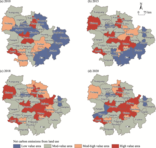
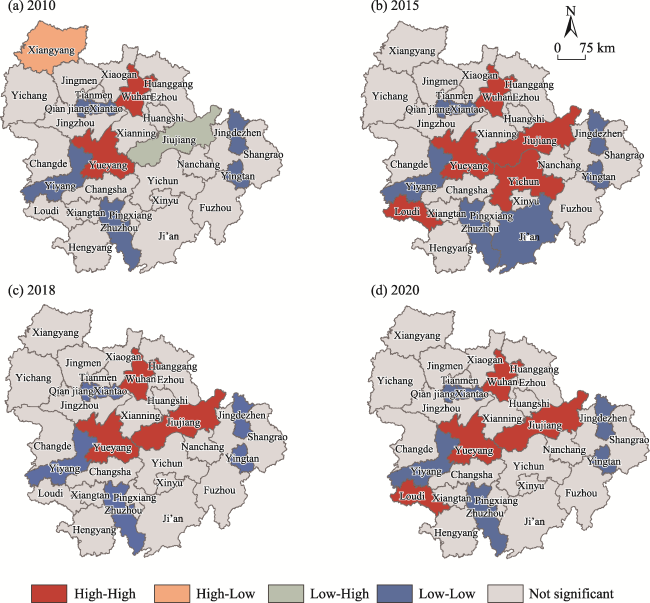
Land use structure is an important factor affecting carbon emissions. Taking the Urban Agglomeration in the Middle Reaches of the Yangtze River (MRYRUA) as an example, this study uses transfer matrix, the carbon emission coefficient method, spatial analyses and geo-detectors to analyze the carbon emission effects of land use changes, as well as their spatial evolutionary characteristics and driving factors, based on the data of 31 cities during 2010-2020. This analysis led to three outcomes. (1) The carbon sinks are insufficient to counterbalance the carbon sources, and net carbon emissions continued to grow from 144.88 million t in 2010 to 160.37 million t in 2020 due to the expansion of construction land. (2) The high-value areas of net carbon emissions shifted from dispersed to concentrated, while low-value areas shifted from concentrated to dispersed and decreased in number. The spatial agglomeration pattern is dominated by High-High agglomeration (H-H) and Low-Low agglomeration (L-L) areas. (3) The spatial differentiation of carbon emissions from land use (LUCEs) is primarily influenced by population density, carbon emission intensity, and technological innovation. Moreover, the interactive effects of land use, energy-efficient technologies, population status, industrial structure, and economic development significantly amplify their individual impacts.

Cite this article

YIN Chuanbin , ZENG Si , LIU Dan . Carbon Emission Effects of Land Use Structure Changes and Their Driving Factors: A Case Study of Urban Agglomeration in the Middle Reaches of the Yangtze River, China[J]. Journal of Resources and Ecology, 2025 , 16(1) : 132 -147 . DOI: 10.5814/j.issn.1674-764x.2025.01.013

1 Introduction

The escalation of carbon emissions profoundly influences extreme weather events and global warming. Consequently, curbing and minimizing carbon emissions has emerged as a pivotal strategy for fostering ecological balance and sustainable regional development (Fan et al., 2018). Land use pattern alterations induced by human activities that result in higher carbon emissions are a key concern in greenhouse gas control. Research spearheaded by the World Resources Organization, along with experts in the carbon cycle, revealed that nearly one-third of all greenhouse gas emissions originate from land use changes, and the CO2 emissions stemming from these changes are the primary driving factors of global climate change and the greenhouse effect (Yi et al., 2011; Meyfroidt et al., 2013). The diversity in land use patterns, coupled with varying speeds and levels of economic development, significantly influence carbon emissions. Optimizing the land use structure can modify the carbon source and sink dynamics to a certain extent, thereby steering the regional society and economy towards a low-carbon transition and sustainable development path (Zeng and Wang, 2015). The volume and efficiency of land use change emissions (LUCEs) are directly linked to achieving carbon neutrality and sustainable economic progress. Consequently, optimizing land use patterns and establishing a sound land use structure are pressing issues that need to be addressed in the context of carbon reduction efforts. Therefore, exploring the carbon emission effect caused by land use changes and analyzing its driving factors are of great significance.
Research on LUCEs has become increasingly prevalent. The effects of LUCEs can be categorized into direct and indirect carbon emission effects, each with distinct mechanisms. Campbell et al. (2000) contended that variations in carbon emissions are significantly affected by land use and subsequent changes in land cover, so they are driven by human activities ranging from deforestation and agricultural practices to the restoration of agricultural land to forest. Those authors also highlighted the influences of increasing CO2 levels and other natural factors, such as climate change. Scott et al. (2010) similarly suggested that CO2 emissions from land use are closely tied to the impact of these practices on regional ecosystem microclimates. Expanding on these insights, Lai (2010) identified three distinct mechanisms of LUCEs in China based on their carbon effects: the natural disturbance mechanism, the transformation mechanism of land use/cover types, and the mechanism involving changes in land management modes. Li (2013) further illuminated how changes in land use types alter carbon emission mechanisms, emphasizing the role of surface vegetation cover in the carbon cycle of ecosystems. He noted that changes in vegetation cover directly affect soil carbon stocks and pointed out that high carbon emissions from land use often result from the irrational allocation of carbon emissions among urban land use types, inefficient land utilization, and the environmental impact of urban planning and industrial layouts.
In the context of accounting for LUCEs and their influencing factors, the scholarly research has been extensive, spanning national, regional, and urban scales. Xing et al. (2019) applied the center of gravity shift model and spatial autocorrelation model to analyze the evolution of the spatial characteristics of LUCEs in China from 2009 to 2016. Ji et al. (2023) conducted a comprehensive assessment of interprovincial LUCEs using data from the Third China National Land Survey. Their work explored not only the structural characteristics and evolutionary process of the spatial correlation network of LUCEs but also included a dynamic analysis of the factors driving these carbon emissions. Similarly, Li et al. (2019) focused on the Yangtze River Delta region and examined the spatial and temporal evolutionary patterns of carbon dioxide emissions, emphasizing the relationship between land use and carbon emissions in this area. Liu et al. (2017) examined the carbon emissions related to land use changes in the Northeast region of China by employing the carbon emission coefficient method and discovered significant pressure from carbon emissions in this region. Hutyra et al. (2011) constructed a land use change matrix for Seattle, USA, from 1986 to 2007, and used it to calculate the carbon emissions or sequestration resulting from transitions between various land types and estimate the total net carbon emissions for Seattle during the study period. Finally, the work of Xu et al. (2016) and Zhou and Zhao (2018) provided urban perspectives by investigating the effects of urban expansion on regional carbon sinks and emissions in Xi'an and Guangzhou City, respectively. All these studies highlighted the localized impact of land-use changes on carbon dynamics.
Despite the extensive amount of research conducted on the carbon emission effects of land use, there is still room for improvement. For example, most studies have focused on the national and urban levels, while relatively few have addressed the regional scale, especially in rapidly developing urban agglomerations. Therefore, this study selected the middle reaches of the Yangtze River urban agglomeration as its research subject to explore the carbon emission effects of land use structure changes and their driving factors. As a typical rapidly developing region, the Urban Agglomeration in the Middle Reaches of the Yangtze River (MRYRUA) is currently in a period of increasing carbon emission pressure due to industrialization and urbanization. Under the dual-carbon goals, accelerating the formation of a low-carbon land use structure in this urban agglomeration is crucial for promoting green and low-carbon economic and social development. This study employed remote sensing image data and socioeconomic data from 31 cities in MRYRUA, and used both direct and indirect carbon emission coefficient methods to assess the carbon sources, carbon sinks, and net carbon emissions of the region, to analyze its spatiotemporal evolutionary characteristics. Simultaneously, this study also employed geographic detectors to analyze the factors driving land use carbon emissions to provide a reference for the regulation of low-carbon land use structures.

2 Theoretical mechanism of LUCEs and research framework

2.1 The carbon emission effect from land use

The carbon emission effect from land use represents the impact of land use activities on regional carbon processes, i.e., the processes and mechanisms through which land use and its changes contribute to the release of atmospheric carbon. This effect can be categorized into direct and indirect effects, depending on the carbon processes and mechanisms involved. The direct effect relates to how land use influences natural carbon processes. In contrast, the indirect effect refers to how land use affects anthropogenic carbon processes, implying that land use activities modify regional carbon dynamics by altering the mode and intensity of human economic activities (Han et al., 2019). Land use changes the mix of human economic activities and energy consumption, thereby altering the intensity and pattern of carbon emissions from land use. Furthermore, the effects of land use on carbon can be both positive and negative. The positive effect manifests in the form of carbon fixation and the augmentation of carbon sinks through land use activities. In contrast, the negative effect involves increased carbon emissions, directly or indirectly, due to land use activities.

2.2 Mechanism of the carbon emission effect from land use

The mechanisms of the direct and indirect effects of land use change differ, each having distinct impact pathways (Han et al., 2019). The direct effect mechanism of LUCEs is affected by changes in land use type and management practices, thereby affecting plant biomass, soil respiration rates, and vegetation carbon sequestration efficiency (Figure 1). On one hand, changes in land use type affect plant biomass and vegetation carbon stocks. Urban expansion, deforestation, the conversion of cropland to forest, agricultural management, and other external natural disturbances and recovery mechanisms, along with changes in surface cover from land use conversions, all impact vegetation carbon storage. On the other hand, these changes also affect soil organic matter inputs and soil conditions, thus influencing the decomposition rate of soil organic carbon and subsequently altering soil carbon stocks. In most cases, changes in land use types affect both vegetation and soil carbon stocks. During industrialization and urbanization, urban expansion and the internal conversion of agricultural land represent the major types of land use changes (Verburg et al., 2015). Urban expansion primarily refers to the expansion of urban construction areas, while the internal conversion of agricultural land typically involves interconversions among forests, grasslands, farmlands, and wetlands (Wang et al., 2022).
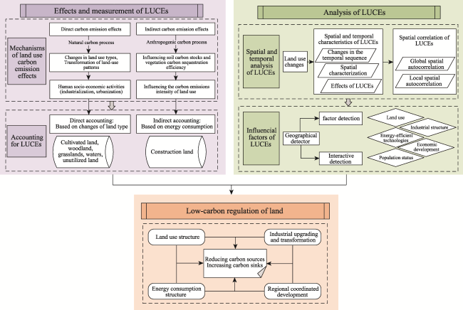
Figure 1 Theoretical framework of this study
The indirect effect mechanism of LUCEs operates primarily through changes in land management practices and human activity-induced carbon emissions. This effect is driven by industrialization and urbanization through changes in the mode and intensity of human socio-economic activities. Different land use types carry different forms of socio-economic activities. Notably, urban areas cover just 2.4% of the global land but account for 80% of global greenhouse gas emissions (Bae and Ryu, 2020). Industrial energy consumption and other activities in urban settings significantly influence carbon emissions. Additionally, the socio-economic and institutional changes spurred by urbanization markedly affect carbon emissions (Yu et al., 2022). In summary, industrialization and urbanization drive profound changes in land use types and socio-economic systems, which in turn significantly affect regional carbon emissions.

2.3 Regulation of land use structure for low-carbon optimization

Analyzing the carbon emission effects of land use is crucial for guiding effective land regulation strategies. The primary goal of land regulation is to reduce the regional carbon emission intensity and improve carbon sequestration levels and efficiency. Optimizing the land use structure is a key tool for achieving this goal (Shu et al., 2019). Different land use modes vary significantly in their carbon source and sink intensities. Regulating land use can reduce the high emission uses, and a differentiated land supply mechanism can lower regional carbon emissions. Optimizing the land use structure to reduce carbon sources or enhance carbon sinks (Zhou et al., 2016; Han et al., 2019) involves constraining urban expansion to achieve carbon emission reduction in construction land on one hand, as well as strengthening the management of ecological lands such as forests, farmlands, grasslands, and wetlands to further increase carbon sequestration on the other hand (Yi et al., 2022).

3 Study area and data sources

3.1 Study area

MRYRUA is a mega-urban agglomeration comprising Wuhan Urban Agglomeration (WHUA), Changsha-Zhuzhou-Xiangtan Urban Agglomeration (CZXUA), and Poyang Lake Urban Agglomeration (PLUA), which encompasses 31 prefectural (county) cities across Hubei Province, Hunan Province and Jiangxi Province (Figure 2). It plays a pivotal role in China’s efforts to promote the development of the Yangtze River Economic Belt, the rise of central China, and the consolidation of the strategic pattern of “two horizontal and three vertical” urbanization. The study region spans 3.17×10⁵ km2, with a population of around 130 million and a GDP of 1.11 trillion yuan, which represented about 9.3% of China’s GDP in 2020.
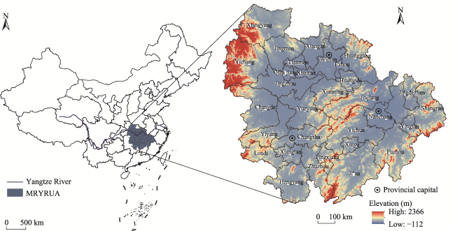
Figure 2 Location of the MRYRUA

3.2 Data sources

Land use data with a spatial resolution of 30 m for the years 2010, 2015, 2018, and 2020 were sourced from the Resource and Environment Science and Data Center of the Chinese Academy of Sciences (https://www.resdc.cn/). The first-level classifications of this dataset include cultivated land, woodland, grassland, water area, construction land and unexploited land. The land use/land cover change (LUCC) data were processed using ArcGIS 10.8, involving reclassification, masking, raster conversion, fusion, and computational geometry to extract the necessary land use data for the study period. The data on energy consumption and other evaluation indicators of the economy, population and industrial structure of each city were obtained from the statistical yearbooks of each city, the statistical bulletins of each city, and the Hubei Statistical Yearbook, Hunan Statistical Yearbook, Jiangxi Statistical Yearbook and China Urban Statistical Yearbook.

4 Research methods

4.1 Methods for calculating carbon emissions from land use

Quantifying the carbon emissions from land use is the basis for analyzing the carbon emission effect from land use. Carbon emissions from land use are affected by both natural ecological processes and socio-economic activities, and a unified accounting method for the carbon emissions from land use is lacking due to the uncertainty of natural ecological processes and the complexity of socio-economic activities (Yi et al., 2022). Currently, a combination of direct and indirect carbon emission calculation methods is widely adopted as the standard practice for estimating land use carbon emissions.

4.1.1 Calculation of direct carbon emission

Forests and grasslands serve as the primary terrestrial carbon sinks, with forests comprising approximately 46% of the global terrestrial carbon pool and grasslands contributing 26% (Watson et al., 2000). Carbon sinks from land use predominantly originate from non-construction areas which encompass cultivated land, woodlands, grasslands, water bodies, and unexploited lands. These areas primarily sequester carbon through vegetation and soil. Consequently, we employed the direct carbon emission calculation method to calculate the carbon emissions from cultivated land, woodland, grassland, waters and unexploited land. The formula is:
$E=\sum\limits_{i=1}^{5}{{{T}_{i}}\times {{\delta }_{i}}}$
where E is the carbon emission from land use (t); Ti is the area of each type of land (ha); δi denotes the carbon emission coefficient of each type of land; and i represents the five land use types. In this study, the carbon emission coefficients of each land use type were combined with the study area and referred to previous studies (Duan et al., 2008; Li et al., 2008; Su and Zhang, 2011; Wan et al., 2017). The carbon emission coefficients of arable land, woodland, grassland, watersheds, and unexploited land were 0.459 t ha-1, -0.644 t ha-1, -0.021 t ha-1, -0.298 t ha-1 and -0.005 t ha-1, respectively. A positive coefficient indicates that the site is a carbon source, while a negative coefficient indicates that the site is a carbon sink.

4.1.2 Calculation of indirect carbon emission

As the core carrier of human production and life, construction land is the main source of carbon. Given that human construction activities significantly affect carbon emissions from construction land, we adopted the indirect carbon emission calculation method to calculate the carbon emissions from construction land and considered eight energy sources: raw coal, coke, natural gas, crude oil, gasoline, kerosene, diesel and electricity. The formula is:
$E=\sum\limits_{i=1}^{8}{{{E}_{i}}\text{ }\!\!\times\!\!\text{ }{{B}_{i}}\text{ }\!\!\times\!\!\text{ }{{\theta }_{i}}}$
where E denotes the carbon emissions from construction land; Ei denotes various forms of energy consumption; Bi denotes the standard coal conversion factor; θi denotes the carbon emission factor; and i denotes the eight types of energy sources. The carbon emission coefficients of the eight types of energy sources were derived from the IPCC Guidelines for National Greenhouse Gas Inventories, and the standard coal conversion coefficients were derived from the China Energy Statistics Yearbook, as shown in Table 1.
Table 1 Standard coal conversion factors and carbon emission factors for the major energy sources
Type of energy Conversion factor for standard coal Carbon emission factor (kg kgce-1)
Raw coal 0.7143 0.7559
Coke 0.9714 0.8550
Natural gas 1.3300 0.4483
Crude oil 1.4286 0.5857
Gasoline 1.4714 0.5538
Kerosene 1.4714 0.5714
Diesel 1.4571 0.5921
Electricity 0.1229 0.7476

Note: In the standard coal conversion factors for major energy sources, the unit of natural gas is kgce m-3, the unit of electricity is kgce kW-1, and the units of the remaining energy sources are kgce kg-1.

4.2 Spatial autocorrelation analysis

The first law of geography indicates that the closer the distance between entities, the stronger their correlation (Tobler, 1970). Spatial autocorrelation includes global spatial autocorrelation and local spatial autocorrelation. To examine the correlations among the cities’ carbon emissions in the study area, we adopted the global Moran’s I index for the global spatial autocorrelation analysis. The global Moran’s I index can only identify the global spatial correlation of carbon emissions in the study area, but it cannot identify the local spatial agglomeration characteristics of carbon emissions in each city. Therefore, we employed the local Moran spatial autocorrelation in our analysis, calculated the local Moran’s I index and plotted the Lisa agglomerations map.

4.3 Geographic detectors

Geographic detectors are a set of statistical methods for detecting spatial heterogeneity and revealing its underlying drivers (Wang and Xu, 2017). The geodetector consists of four parts: factor detection, risk detection, ecological detection and interaction detection, which can overcome the problem of multicollinearity in traditional econometric regression. Therefore, we used factor detection and interaction detection to explore the drivers of carbon emissions in the study area. Factor detection was mainly used to detect the spatial heterogeneity of carbon emissions and the degree of influence of each influencing factor on the spatial heterogeneity of carbon emissions. The factor detection expression is:
$q=1-\frac{\sum\limits_{h=1}^{L}{{{N}_{h}}\sigma _{h}^{2}}}{N{{\sigma }^{2}}}$
where the q quantifies the influence of a factor on the spatial differentiation of carbon emissions, with q values ranging from 0 to 1. A larger q value signifies greater explanatory power of the driving factor on the spatial differentiation of carbon emissions, while a lower q value indicates weaker explanatory power. For the other variables, h denotes the number of strata of the detecting factor; Nh denotes the number of cities in stratum h; σh2 denotes the variance of the carbon emissions in stratum h; N denotes the number of cities; and σ2 denotes the variance of the carbon emissions of the whole study area.
To identify the interactions between different drivers, we used interaction probes to assess whether the explanatory power of the spatial differentiation of carbon emissions is enhanced or weakened when the drivers interact in pairs. The results are manifested in five relationships: when q(X1∩X2)< Min[q(X1), q(X2)], the interaction between the two factors shows nonlinear attenuation; when Min[q(X1), q(X2)]< q(X1∩X2)<Max[q(X1), q(X2)], it indicates nonlinear attenuation of a single factor; when q(X1∩X2)>Max[q(X1), q(X2)], the interaction between the two factors shows two-factor enhancement; when q(X1∩X2)=q(X1)+q(X2), the two factors are independent; and when q(X1∩X2)>q(X1)+q(X2), the two-factor interaction shows nonlinear enhancement (Wang and Xu, 2017).

5 Results and analysis

5.1 Changes in land use structure

5.1.1 Overall change in the land use structure of MRYRUA

We processed the 30 m-resolution land use remote sensing data from the Resource and Environment Science and Data Center of the Chinese Academy of Sciences using ArcGIS, and after reclassification, we calculated the areas of various land types in MRYRUA for the years 2010, 2015, 2018, and 2020. Table 2 presents the data on changes in the land use structure of MRYRUA between 2010 and 2020, and notable shifts occurred in the area of each land type within the region during this period. Specifically, the rates of change for construction land and grassland exhibited positive trends. The rate of change for construction land amounted to 24.18%, resulting in a substantial increase from 2010 to 2020, with an expansion of 2869 km2. Meanwhile, the grassland area increased from 8772 km2 to 8952 km2, for a change rate of 2.05%. In contrast, other land types experienced negative growth over this period. The area of waters declined from 22981 km2 to 22555 km2, representing a change rate of -1.85%. Unexploited land also decreased, contracting from 1910 km2 to 1883 km2, for a change rate of -1.41%. Woodland exhibited a reduction from 173864 km2 in 2010 to 172327 km2 in 2020, for a change rate of -0.88%. Lastly, the cropland area declined from 123235 km2 to 122160 km2, resulting in a change rate of -0.87%. The rates of change for each land type, arranged from highest to lowest, are as follows: construction land>grassland>water area>unexploited land>woodland>cultivated land. Thus, the transformation in the land use structure can be primarily attributed to the processes of industrialization and urbanization. The rapid economic development of MRYRUA has led to a growing demand for construction land, prompting the conversion of significant amounts of cultivated land, woodland, and water area into construction land.
Table 2 Changes in the land use structure of MRYRUA, 2010-2020 (Unit: km2)
Land type Year Urban agglomeration
PLUA WHUA CZXUA MRYRUA
Grassland 2010 2475 1431 1364 8772
2015 2458 1424 1356 8723
2018 2550 1425 1356 9006
2020 2536 1435 1340 8952
Rate of change (%) 2.46 0.28 -1.76 2.05
Cultivated land 2010 22934 29011 33751 123235
2015 22715 28603 33511 122029
2018 22466 28323 33174 120899
2020 22448 28991 33146 122160
Rate of change (%) -2.12 -0.07 -1.79 -0.87
Construction land 2010 2042 3962 2884 11867
2015 2403 4469 3308 13710
2018 2842 4786 3836 15387
2020 2857 4303 3880 14736
Rate of change (%) 39.91 8.61 34.54 24.18
Woodland 2010 43028 20261 52067 173864
2015 42910 20172 51873 173295
2018 42629 20140 51670 172412
2020 42618 20216 51679 172327
Rate of change (%) -0.95 -0.22 -0.66 -0.88
Water area 2010 5614 6584 5783 22981
2015 5624 6584 5803 22978
2018 5617 6563 5803 22996
2020 5642 6280 5814 22555
Rate of change (%) 0.50 -4.62 0.54 -1.85
Unexploited land 2010 542 165 979 1910
2015 524 162 978 1888
2018 528 158 987 1894
2020 528 186 966 1883
Rate of change (%) -2.58 12.73 -1.33 -1.41
The Sankey diagram of the land use structure changes in MRYRUA from 2010 to 2020 (Figure 3) shows that MRYRUA is primarily composed of woodland and cultivated land, followed by water area, construction land, grassland, and unexploited land. Over the decade spanning from 2010 to 2020, the areas of cultivated land and woodland experienced slight reductions. Specifically, cultivated land was mainly converted into woodland, construction land, and waters, while woodland was primarily shifted to cultivated land and construction land. Nevertheless, cultivated land and woodland combined still accounted for 86% of MRYRUA’s total land area in 2020. During this period, the construction land area generally increased, albeit with some fluctuations and occasional declines. Its growth primarily stemmed from cultivated land and woodland. Grassland generally expanded, with most of the new grassland originating from woodland and cultivated land. Meanwhile, the area of water areas decreased, with the majority of this reduction occurring in cultivated land. Additionally, the unexploited land area decreased, primarily due to conversions into water area and cultivated land.
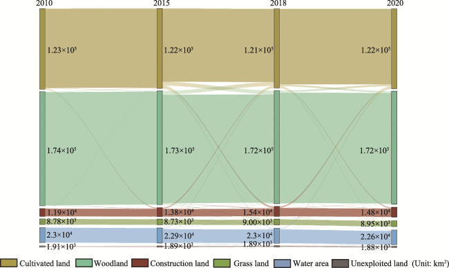
Figure 3 Sankey diagram of land use structure changes

5.1.2 Changes in land use structure of the sub-urban agglomerations

The land use structures show significant differences among the three sub-urban agglomerations. From 2010 to 2020, the cultivated land and grassland of each sub-urban agglomeration showed negative growth, whereas construction land saw a significant increase, indicating growth. The advancement of urbanization and industrialization has made the populations of the cities expand continuously, resulting in a rapidly growing demand for construction land. The construction land growth rates for the three sub-urban agglomerations rank as follows: PLUA (39.91%)>CZXUA (34.54%)> WHUA (8.61%).
Variations in economic development and topographical features among the sub-urban agglomerations led to significant differences in the directions of land use structure changes. These differences were primarily observed in grassland, water area, and unexploited land. In PLUA and WHUA, grassland areas saw positive rates of change, suggesting expansion. In contrast, CZXUA experienced a reduction in grassland area. Regarding water areas, WHUA experienced a significant reduction, with a change rate of -4.62%. However, PLUA and CZXUA saw increases in their water areas. The unexploited land area of WHUA increased significantly, while PLUA and CZXUA saw reductions of 2.58% and 1.33%, respectively.

5.2 Analysis of carbon emissions from land use

5.2.1 Temporal evolution of carbon emissions in MRYRUA

We took the prefecture-level cities of MRYRUA as the evaluation units. Employing both the direct and indirect carbon emission calculation methods, we comprehensively calculated the carbon emissions for each land type in each city for the years 2010, 2015, 2018, and 2020. Subsequently, we derived the LUCEs for both MRYRUA and its sub-urban agglomerations by summing them up. Figure 4 shows the changes in the LUCEs of MRYRUA from 2010 to 2020.
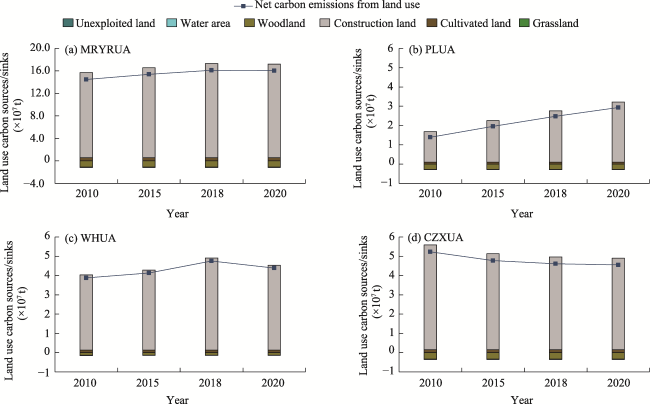
Figure 4 Carbon emissions from land use in each urban agglomeration

Note: “+” indicates carbon sources, “-” indicates carbon sinks.

Figure 4a shows the intrinsic structure and changes in carbon emissions from land use in MRYRUA. Construction land and cultivated land are the main carbon sources, while woodland and water area are the main land types of carbon sinks. The carbon emissions from construction land are 14 times greater than the carbon absorption by woodland, and the net carbon emissions show an overall increasing trend. The total carbon emission rose from 156.82 million tons in 2010 to 172.19 million tons in 2020, an increase of 9.8%. The total carbon absorption declined from 11.94 million tons in 2010 to 11.82 million tons in 2020, indicating a gradual decrease in MRYRUA’s carbon absorption capacity. The continuous expansion of construction land area along with reductions in water area and woodland suggest that MRYRUA’s land carbon sources are growing while the carbon sinks are diminishing, resulting in a net carbon emission increase from 144.88 million tons in 2010 to 160.37 million tons in 2020, or a 10.7% rate of change. This means that MRYRUA is still far from achieving carbon neutrality.
Figure 4b-4d shows the intrinsic structure and changes in LUCEs of the sub-urban agglomerations, and clearly indicates differences in the land-use carbon emissions among the sub-urban agglomerations. The net carbon emission of PLUA gradually increased, the net carbon emission of WHUA increased at first and then decreased, and the net carbon emission of CZXUA gradually decreased. The changes in the net carbon emissions of the sub-urban agglomerations are consistent with the changes in the construction land. On one hand, the growing demand for construction land driven by economic development led to the encroachment on numerous carbon sink lands such as woodland and water area. On the other hand, irrational land use practices have severely damaged ecosystem structures and functions, affecting the carbon storage capacity of the ecosystems.
In general, the carbon source effect from construction land in MRYRUA is relatively significant, while the carbon sink effects from woodland, grassland, water area and unexploited land are not significant. Thus, the carbon sinks are insufficient to counterbalance the carbon sources, so managing the growth of construction land to limit the increase in carbon sources is a critical concern for the future urban development of MRYRUA.

5.2.2 Spatial evolution of carbon emissions in MRYRUA

We adopted the natural breakpoint method to classify the net carbon emissions from land use into four levels: high net carbon emissions area, mod-high net carbon emissions area, moderate net carbon emissions area and low net carbon emissions area, as shown in Figure 5. Overall, there are significant spatial differences in the carbon emissions in MRYUA. The net carbon emission characteristics of each city and agglomeration changed significantly. The distribution of high-value areas of net carbon emissions in MRYRUA changed from scattered to concentrated, with the quantity increasing at first and then decreasing. Conversely, the distribution of the mod-high-value areas shifted from concentrated to scattered, with their quantity decreasing initially and then increasing. The mod-value areas maintained a relatively centralized distribution and experienced an increase in quantity. The low value areas changed from being scattered to concentrated, and their quantity decreased. The increase in the number of high value areas and the reduction in the number of low value areas indicate the growing pressure for carbon emission reduction in MRYRUA.
Figure 5 Spatial distribution of net carbon emissions by city in MRYRUA, 2010-2020
Specifically, from 2010 to 2015, Yichang and Yichun cities experienced increases in carbon emissions from land use, which shifted them from the mod-high-value zone to the high-value zone. Xiangtan City, Hengyang City, Huangshi City, and Jiujiang City moved from the mod-value zone to the mod-high-value zone. Qianjiang City, Jingzhou City, Xianning City, Tianmen City, Huanggang City, and Shangrao City moved from the low-value zone to the mod-value zone. Only Zhuzhou City shifted from the mod-value zone to the low-value zone. During this period, seven cities transitioned to higher net carbon emission zones, and one city moved to a lower net carbon emission zone. These changes suggested that MRYRUA has experienced a notable increase in carbon sources, which resulted in a significant rise in net carbon emissions. From 2015-2018, Huangshi City and Jiujiang City shifted from the medium-high-value zone to the high-value zone. Xiaogan City, Huanggang City, Nanchang City and Xiangtan City shifted from the mod-value zone to the mod-high-value zone. Yingtan City, Fuzhou City, Ji'an City and Zhuzhou City shifted from the low value zone to the mod-value zone. Only Pingxiang City shifted from the mod-high value zone to the mod-value zone. In this stage, 11 cities shifted to a higher net carbon emission zone, and one city shifted to a lower net carbon emission zone, indicating that the carbon sources of MRYRUA continuously increased and the carbon emission reduction situation was severely inadequate. From 2018-2020, Ezhou City shifted from the mod-value zone to the mod-high-value zone. Yiyang City shifted from the mod-value zone to the low-value zone. Yichang City, Huangshi City, Huanggang City, and Yiyang City all dropped to the lower net carbon emission zone, indicating that the growth of carbon sources in MRYRUA had slowed down in this period, and the pressure for carbon emission reduction had eased.

5.2.3 Analysis of carbon emission effects in MRYRUA

To further investigate the carbon emission effects of land use in MRYRUA, we analyzed the carbon emission intensity by calculating the Carbon Emission Per Unit Land Area (CEPL) and the Carbon Emission Per Unit GDP (CEPG) of MRYRUA and each sub-urban agglomeration (Figure 6). From 2010-2020, MRYRUA’s CEPL increased from 423 t km-2 in 2010 to 468 t km-2 in 2020, for an increase of 10.7%. MRYRUA’s CEPG decreased from 0.41 t (104 yuan)-1 in 2010 to 0.17 t (104 yuan)-1 in 2020, for a reduction of 59%. This means that as economic development progressed and the land use structures changed, MRYRUA’s carbon emission pressure rose incrementally, yet its carbon emission efficiency also improved.
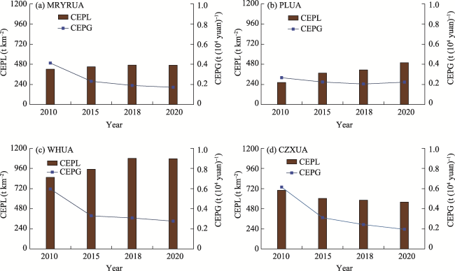
Figure 6 The trends of changes in CEPL and CEPG
There are significant differences in CEPL and CEPG among the three sub-urban agglomerations. In terms of CEPL, the descending order ranking of the three sub-urban agglomerations in 2020 was WHUA>CZXUA>PLUA. Although PLUA had the lowest CEPL, it experienced the fastest growth rate, with an increase of 90% from 262 t km-2 in 2010 to 498 t km-2 in 2020. WHUA had the highest CEPL, averaging 989 t km-2. Although it declined after 2018, it still increased by 26% during the study period. CZXUA’s CEPL gradually declined from 699 t km-2 in 2010 to 558 t km-2 in 2020, a 20% reduction. In terms of CEPG, the descending order ranking of the three sub-urban agglomerations in 2020 was WHUA>PLUA>CZXUA. From 2010-2020, the CEPG of the three urban agglomerations showed downward trends. The CEPG of WHUA, PLUA and CZXUA declined from 0.60, 0.27 and 0.61 t (104 yuan)-1 in 2010 to 0.28, 0.22 and 0.20 t (104 yuan)-1 in 2020, respectively, for reductions of 53.7%, 16.3% and 63.1%, respectively.

5.3 Analysis of spatial variance

5.3.1 Global spatial autocorrelation analysis

To further reveal the spatial distribution characteristics, we applied Geoda software to carry out the global Moran analysis and local Moran analysis on the net carbon emissions of MRYRUA cities for the years of 2010, 2015, 2018 and 2020. As shown in Table 3, the global Moran’s I indices of net carbon emissions from land use in the study area from 2010 to 2020 were all greater than 0 and statistically significant (P<0.05), with Z-scores exceeding 2.58. These results indicated a positive spatial agglomeration of net carbon emissions in MRYRUA overall, in which the high-emission regions were contiguous with other high-emission regions, and low-emission regions were contiguous with other low-emission regions.
Table 3 Global spatial autocorrelation of Moran’s I values of net land use carbon emissions in MRYRUA
Variable 2010 2015 2018 2020
Global Moran’s I index 0.404 0.596 0.6367 0.7211
Z-score value 4.2192 6.1875 6.6582 7.4649
P value 0.004 0.001 0.001 0.001

5.3.2 Local spatial autocorrelation analysis

We conducted a local Moran spatial autocorrelation analysis to reveal the local spatial correlation patterns of net carbon emissions among the cities in MRYRUA. As shown in Figure 7, the spatial agglomeration patterns of net carbon emissions in the MRYRUA cities were dominated by High-High agglomeration and Low-Low agglomeration. From 2010 to 2020, the High-High agglomeration areas expanded, and were predominantly situated in the central region of the study area, while the number of Low-Low agglomerations remained unchanged and they were scattered in the eastern and southwestern regions. More specifically, High-High agglomeration was primarily concentrated in cities like Wuhan City, Yueyang City, Loudi City, Jiujiang City, and Yichun City. These cities boast relatively developed economies and expansive construction land areas, leading to higher carbon emissions. On the other hand, Low-Low agglomeration was predominantly observed in cities such as Qianjiang City, Xiantao City, Yiyang City, Zhuzhou City, Jingdezhen City, and Yingtan City. These cities are characterized by vast forested regions, limited land allocated for construction, and economies primarily focused on tourism and light industry, resulting in lower carbon emissions.
Figure 7 LISA maps of the spatial agglomeration of net carbon emissions in MRYRUA, 2010-2020

5.4 Analysis of the factors driving carbon emissions

5.4.1 Selection of driving factors

Drawing on existing related studies, we selected 10 indicators from the factor layers of land use, energy-saving technology, population status, industrial structure, and economic development to determine which factors influence carbon emissions in the study area. The indicator system of the driving factors is shown in Table 4.
Table 4 Indicators of carbon emission driving factors
Elementary layer Indicator layer Description of the indicator
Land use X1 Degree of land use Construction land area/Total area
X2 Land use efficiency Gross domestic product/Built-up land area
Energy-efficient technologies X3 Energy consumption structure Coal use/Total energy use
X4 Technological innovation Number of patents granted
X5 Carbon emission intensity Carbon emissions/Gross domestic product
Population status X6 Population urbanization Urban population/Total population
X7 Population density Total population/Total area
Industrial structure X8 Industrial structure Second industry output/Output of the tertiary industry
Economic development X9 Per capita GDP Gross domestic product/Total population
X10 Per capita total retail sales Total retail sales/Total population
For the aspect of land use, we mainly considered the land use degree (Xu et al., 2016) and land use efficiency (Han et al., 2019). Given that construction land is the main source of carbon emissions, we used the ratio of construction land area to regional land area to reflect the land use degree, and the ratio of regional GDP to construction land area to reflect land use efficiency. In terms of energy-efficient technologies, we mainly considered the energy consumption structure (Xu et al., 2014), the level of technological innovation (Lewis, 2016), and carbon emission intensity. We used the proportion of coal use in total energy use to reflect the energy consumption structure, the number of patents granted to reflect the level of technological innovation, and the carbon emission intensity was calculated by dividing the carbon emissions by the regional GDP. For the aspect of population status factors, we mainly considered the level of population urbanization and population density (Ou et al., 2016; He et al., 2019), which are reflected by the proportion of the urban population to the total population of the region and the proportion of the total population to the total area of the region, respectively. In terms of industrial structure (Zhou et al., 2013; Han and Shao, 2022), we adopted the ratio of second industry output to the output of the tertiary industry to reflect this. For the aspect of economic development factors, we considered the level of production and the level of consumption together, and used per capita GDP (Hannesson, 2019) and per capita total social retail sales (Wang et al., 2016; Li et al., 2021) to reflect them, respectively.

5.4.2 Optimizing parameter discretization of the continuous factors

Since the geographical detector excels at analyzing categorical variables, we calculated and compared them to obtain the maximum q-value of each continuous variable under different classification methods, and then detected the explanatory power of each driving factor on the spatial differentiation of carbon emissions. We discretized each continuous factor in 2010, 2015, 2018, and 2020 by the natural breakpoint method, quantile breakpoint method, geometrical interval method, and equal division method to find the maximum q-value, and a larger value indicates a better discretization effect. Then we obtained the optimal discretization method for each factor in the different years.
As shown in Figure 8, the different discretization methods have different discretization effects on each driving factor. The discretization method that yields the maximum q-value was selected as the optimal parameter for each factor. Taking the degree of land use as an example, the q-value of the natural breakpoint method was the largest in 2010 and 2018, but the q-value of the geometric interval method was the largest in 2015 and 2020. Therefore, the natural breakpoint classification was used as the optimal parameter selection method in 2010 and 2018, and the geometric interval classification was used as the optimal parameter selection method in 2015 and 2020. The other driving factors were analyzed similarly.
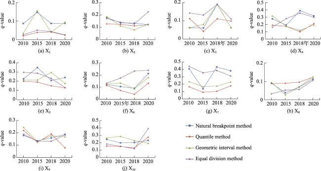
Figure 8 Discretized q-values of the continuous driving factors

5.4.3 Factor detection analysis

Table 5 shows the results of the factors influencing the spatial differentiation of carbon emissions in the study area from 2010 to 2020. Considering the influence of each factor, the spatial differentiation of carbon emissions results from the combined effect of multiple factors. Over different periods, the core factors driving the spatial differentiation of carbon emissions in the study area exhibited both consistency and variability. The top three core drivers in 2010 were X7 population density (0.441), X4 technological innovation (0.318), and X5 carbon emission intensity (0.296); the top three core drivers in 2015 were X7 population density (0.354), X5 carbon emission intensity (0.348), and X4 technological innovation (0.280); the top three core drivers in 2018 were X7 population density (0.433), X4 technological innovation (0.390), and X5 carbon emission intensity (0.296); and the top three core drivers in 2020 were X7 population density (0.381), X4 technological innovation (0.317), and X5 carbon emission intensity (0.240). Averaged over all the periods, the top three core drivers were X7 population density (0.402), X4 technological innovation (0.326), and X5 carbon emission intensity (0.295). Clearly these three factors were the main drivers of the spatial differentiation of carbon emissions in MRYRUA.
Table 5 Detection results of factors driving the spatial differentiation of carbon emissions in MRYRUA, 2010-2020
Year Influence q-value
X1 X2 X3 X4 X5 X6 X7 X8 X9 X10
2010 0.087 0.187 0.143 0.318 0.296 0.133 0.441 0.095 0.245 0.266
2015 0.157 0.141 0.132 0.280 0.348 0.176 0.354 0.091 0.135 0.288
2018 0.087 0.133 0.190 0.390 0.296 0.234 0.433 0.096 0.190 0.231
2020 0.094 0.225 0.110 0.317 0.240 0.240 0.381 0.125 0.186 0.132
Mean 0.106 0.172 0.144 0.326 0.295 0.196 0.402 0.102 0.189 0.229

5.4.4 Analysis of interactions

The results of pairwise interactions among the 10 factors are shown in Figure 9. The explanatory power of the pairwise interaction of driving factors exceeds that of the individual factors. The interaction patterns are characterized by enhancement and nonlinear enhancement, with no independent or weakening effects. In general, the q-values of the pairwise interactions are all greater than 0.3, indicating that the spatial distribution of carbon emissions is a result of the combined effects of these factors.
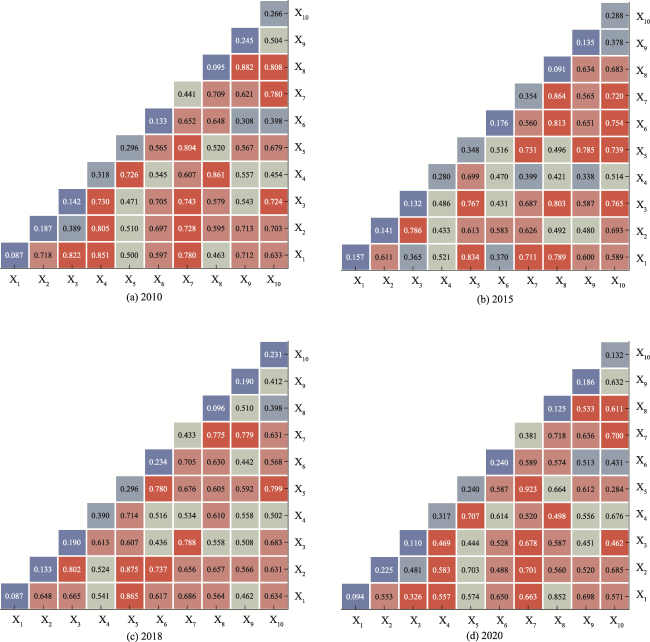
Figure 9 Interaction results of the factors driving the spatial differentiation of carbon emissions in MRYRUA, 2010-2020
In 2010, the seven interactions of X8 industrial structure∩X9 per capita GDP (0.882), X8 industrial structure∩X4 technological innovation (0.861), X1 land use degree∩X4 technological innovation (0.851), X1 land use degree∩X3 energy consumption structure (0.822), X7 population density∩X10 per capita total retail sales (0.808), X2 land use efficiency∩X4 technological innovation (0.805) and X5 carbon emission intensity∩X7 population density (0.804) played major roles in the spatial differentiation of carbon emissions. In addition, the interaction between X7 population density and its remaining factors also played an obvious role in the spatial differentiation of carbon emissions, and the q-value of this interaction was greater than 0.6, indicating that the influence of population density and other factors on the spatial distribution of carbon emissions in the study area was significantly enhanced by the spatial superposition of these two factors.
In 2015, the X8 industrial structure played a major role in the spatial differentiation of carbon emissions after interacting with the remaining factors. The interaction between X8 industrial structure and X7 population density amounted to 0.864, while the interaction with X6 population urbanization was 0.813, and the interaction with X3 energy consumption structure was 0.803. In addition, the interaction between X1 land use degree and X5 carbon emission intensity was 0.834, so it also contributed to the spatial differentiation of carbon emissions.
In 2018, the interaction between X2 land use efficiency and X5 carbon emission intensity was the largest, reaching 0.875. In addition, the interactions of X1 land use degree∩X5 carbon emission intensity (0.865), and X2 land use efficiency∩X3 energy consumption structure (0.802) were also important. These results indicated that pairwise interactions between land use efficiency and carbon emission intensity, land use degree and carbon emission intensity, and land use efficiency and energy structure had significant impacts on the spatial differentiation of carbon emissions.
In 2020, the interactions between X7 population density and other factors all exceeded 0.5, playing a major role in the spatial differentiation of carbon emissions. The interaction between X7 population density and X5 carbon emission intensity reached as high as 0.923. In addition, the interaction between X1 land use degree and X8 industrial structure was 0.852. These results indicated that the spatial superpositions of population density∩carbon emission intensity and land use degree∩industrial structure played a dominant role in the spatial distribution of carbon emissions in the study area.

6 Conclusions

The conclusions of this study are as follows.
First, the land use structure of MRYRUA underwent substantial changes from 2010-2020. These changes were characterized by reductions in the acreage devoted to arable land, forested areas, and bodies of water, coupled with the expansion of grassland, construction zones, and unexploited land. The construction land areas in PLUA, WHUA and CZXUA all significantly increased. Cultivated land and woodland were the main sources of new construction land. The carbon sinks provided by land were insufficient to counterbalance the carbon sources from land use, resulting in a consistent increase in net carbon emissions in MRYRUA. The expansion of construction land was the main reason for the increase in net carbon emissions.
Second, there were significant spatial differences in net carbon emissions from land use among the different cities in MRYRUA. The number of high-value areas for net carbon emissions increased and tended to be clustered, while the number of low-value areas decreased and became more dispersed. The spatial agglomeration pattern of net carbon emissions was dominated by High-High agglomeration and Low-Low agglomeration. The High-High agglomeration areas showed a trend of expansion, and were mainly distributed in the central part of the study area, while the number of Low-Low agglomeration areas remained constant, and they were scattered in the eastern and southwestern parts of the study area.
Third, the factors driving the spatial differences in land use carbon emission effects within MRYRUA were complex, resulting from both the independent effects of various factors and their interactions. Population density, carbon emission intensity, and technological innovation factors were the main drivers, while the influence of pairwise interactions between factors such as land use, energy-efficient technologies, population status, industrial structure, and economic development significantly increased.
[1]
Bae J, Ryu Y. 2020. High soil organic carbon stocks under impervious surfaces contributed by urban deep cultural layers. Landscape and Urban Planning, 204(1): 103953. DOI: 10.1016/j.landurbplan.2020.103953.

[2]
Campbell C A, Zentner R P, Liang B C, et al. 2000. Organic C accumulation in soil over 30 years in semiarid southwestern Saskatchewan—Effect of crop rotations and fertilizers. Canadian Journal of Soil Science, 80(1): 179-192.

[3]
Duan X N, Wang X K, Lu F, et al. 2008. Current status and potential of carbon sequestration in wetland ecosystems in China. Acta Ecologica Sinica, 28(2): 463-469. (in Chinese)

[4]
Fan J S, Yu X F, Zhou L. 2018. Carbon emission efficiency growth of land use structure and its spatial correlation in Nanjing. Geography Research, 37(11): 2177-2192. (in Chinese)

[5]
Han X, Cao T, Sun T. 2019. Analysis on the variation rule and influencing factors of energy consumption carbon emission intensity in China’s urbanization construction. Journal of Cleaner Production, 238(20): 117958. DOI: 10.1016/j.jclepro.2019.117958.

[6]
Han Y, Shao Y. 2022. Impact mechanisms of carbon emissions, industrial structure and environmental regulations in the Yellow River Basin. Polish Journal of Environmental Studies, 31(6): 5693-5709.

[7]
Hannesson R. 2019. CO2 intensity and GDP per capita. IAEE International Conference: May 29-June 1, 2019. Montreal, Canada: International Association for Energy Economics: 1-23.

[8]
He W J, Zhang H F, Chen X C, et al. 2019. An empirical study on population density, industrial agglomeration and carbon emission in China: from the perspective of agglomeration economy, crowding effect and spatial effect. Nankai Economic Research, (2): 207-224. (in Chinese)

[9]
Hutyra L R, Yoon B, Hepinstall-Cymerman J, et al. 2011. Carbon consequences of land cover change and expansion of urban lands: A case study in the Seattle Metropolitan region. Landscape & Urban Planning, 103(1): 83-93.

[10]
Ji X Q, Liu H M, Zhang Y S. 2023. Evolution and driving factors of spatial association network structure of carbon emissions from provincial land use in China. Economic Geography, 43(2): 190-200. (in Chinese)

[11]
Lai L. 2010. Carbon emission effects of land use in China. Diss., Nanjing, China: Nanjing University. (in Chinese)

[12]
Lewis N S. 2016. Aspects of science and technology in support of legal and policy frameworks associated with a global carbon emissions-control regime. Energy & Environmental Science, 9(7): 2172-2176.

[13]
Li J B, Huang X J, Sun S C, et al. 2019. Spatiotemporal coupling analysis of CO2 emissions from urban land and energy consumption in Yangtze River Delta. Geographical Research, 38(9): 2188-2201. (in Chinese)

[14]
Li K Q. 2013. A study on the evaluation and structural optimization of regional land use oriented to low carbon economy. Diss., Wuhan, China: Huazhong Agricultural University. (in Chinese)

[15]
Li R, Wang Q, Liu Y, et al. 2021. Per-capita carbon emissions in 147 countries: The effect of economic, energy, social, and trade structural changes. Sustainable Production and Consumption, 27(8). DOI: 10.1016/j.spc.2021.02.031.

[16]
Li Y, Huang X J, Zhen F. 2008. Analysis of carbon emission effects of different land use patterns in Jiangsu Province. Journal of Agricultural Engineering, 24(S2): 102-107. (in Chinese)

[17]
Liu X R, Yang L, Wang Y, et al. 2017. Study on carbon emission effects based on land use change in northeast China. Soil and Water Conservation Bulletin, 37(2): 107-114. (in Chinese)

[18]
Meyfroidt P, Lambin E F, Erb K H, et al. 2013. Globalization of land use: Distant drivers of land change and geographic displacement of land use. Current Opinion in Environmental Sustainability, 5(5): 438-444.

[19]
Ou J P, Liu X P, Li X, et al. 2016. Mapping global fossil fuel combustion CO2 emissions at high resolution by integrating nightlight, population density, and traffic network data. IEEE Journal of Selected Topics in Applied Earth Observations & Remote Sensing, 9(4): 1674-1684.

[20]
Scott N A, Tate K R, Ford-Robertson J, et al. 2010. Soil carbon storage in plantation forests and pastures: Land-use change implications. Tellus Series B—Chemical & Physical Meteorology, 51(2): 326-335.

[21]
Shu H, Xiong P P. 2019. Reallocation planning of urban industrial land for structure optimization and emission reduction: A practical analysis of urban agglomeration in China’s Yangtze River Delta. Land Use Policy, 81: 604-623.

DOI

[22]
Su Y L, Zhang Y F. 2011. Study on carbon emission benefits of land use change in Shaanxi Province. Journal of Soil and Water Conservation, 25(1): 151-156. (in Chinese)

[23]
Tobler R W. 1970. A computer movie simulating urban growth in the Detroit Region. Economic Geography, 46: 234-240.

[24]
Verburg P H, Crossman N, Ellis E C, et al. 2015. Land system science and sustainable development of the earth system: A global land project perspective. Anthropocene, (12): 29-41.

[25]
Wan W, Wei W, Qian D, et al. 2017. Research progress on environmental effects of land use/cover change. Journal of Fujian Agriculture and Forestry University: Natural Science Edition, 46(4): 361-372. (in Chinese)

[26]
Wang J F, Xu C D. 2017. Geo-detectors: Principles and prospects. Acta Geographica Sinica, 72(1): 116-134. (in Chinese)

[27]
Wang W, Zou W, Zhang G, et al. 2022. Urban agglomeration land spatial planning path and governance mechanism under “Double Carbon” goal. Environmental Protection, 50(1): 64-69. (in Chinese)

[28]
Wang X S, Ren S G, Yuan B L, et al. 2016. Effects of urbanization, urban-rural consumption ratio and structure on indirect CO2 emissions from household consumption. Economic Theory and Economic Management, (8): 79-88. (in Chinese)

[29]
Watson R T, Noble I R, Bolin B, et al. 2000. Land use, land-use change, and forestry:A special report of the IPCC. Cambridge, UK: Cambridge University Press.

[30]
Xing X W, Li X D, Huang X, et al. 2019. Study on the evolution of spatial characteristics of carbon emissions from land use in China. Resource Development and Market, 35(11): 1351-1361. (in Chinese)

[31]
Xu Q, Yang R, Dong Y X, et al. 2016. The influence of rapid urbanization and land use changes on terrestrial carbon sources/sinks in Guangzhou, China. Ecological Indicators, 70(11): 304-316.

[32]
Xu S C, He Z X, Long R Y. 2014. Factors that influence carbon emissions due to energy consumption in China: Decomposition analysis using LMDI. Applied Energy, 127(8): 182-193.

[33]
Yi D, Ou M H, Guo J, et al. 2022. Progress and trend of carbon emission from land use and low carbon optimization. Resources Science, 44(8): 1545-1559. (in Chinese)

[34]
Yi W J, Zou L L, Guo J, et al. 2011. How can China reach its CO2 intensity reduction targets by 2020? A regional allocation based on equity and development. Energy Policy, 39(5): 2407-2415.

[35]
Yu Q Y, Li M, Li Q, et al. 2022. Economic agglomeration and emissions reduction: Does high agglomeration in China’s urban clusters lead to higher carbon intensity? Urban Climate, 43: 101174. DOI: 10.1016/J.UCLIM.2022.101174.

[36]
Zeng Y N, Wang W M. 2015. Optimization scheme of land use structure in Haidong City targeting low carbon. Resources Science, 37(10): 2010-2017. (in Chinese)

[37]
Zhou X, Zhang M, Zhou M, et al. 2016. A comparative study on decoupling relationship and influence factors between China’s regional economic development and industrial energy-related carbon emissions. Journal of Cleaner Production, 142(2): 783-800.

[38]
Zhou X Y, Zhang J, Li J P. 2013. Industrial structural transformation and carbon dioxide emissions in China. Energy Policy, 57(6): 43-51.

[39]
Zhou Y, Zhao W. 2018. Carbon emission accounting and low carbon optimization of land use structure in Xi’an City. Ecoeconomics, 34(5): 21-25. (in Chinese)

Outlines

/