
Journal of Resources and Ecology >
Two-sided and Heterogeneous Effects of Environmental Regulation on the Technological Innovation Efficiency of Iron and Steel Enterprises in China
|
GE Zehui, E-mail: gezehui@ustb.edu.cn |
Received date: 2023-09-01
Accepted date: 2024-03-20
Online published: 2024-12-09
Supported by
The National Natural Science Foundation of China(71871016)
The Fundamental Research Funds for the Central Universities(FRF-DF-20-68)
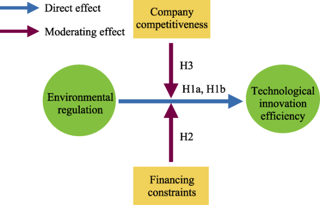
In this study, the relationship between environmental regulations and technological innovation efficiency is empirically examined via panel data from 33 iron and steel enterprises (ISs) in China between 2015 and 2021. The results show that the average “innovation compensation effect” of environmental regulations on the technological innovation efficiency of ISs exceeds the average “compliance cost effect”, thus resulting in a clearly positive net effect. Both the two-sided effects and the net effects vary across different years, geographical regions, and types of property rights. As the quantile of technological innovation efficiency increases, the positive influence of environmental regulations tends to increase. Furthermore, the strengthening of financing constraints and firm competitiveness enhances the positive impact of environmental regulations on the technological innovation efficiency of ISs. Additionally, a double-threshold effect of environmental regulations on the technological innovation efficiency of ISs is revealed in this study. The realisation of the Porter hypothesis occurs when financing constraints and firm competitiveness fall within specific threshold intervals. This research not only deepens our understanding of the relationship between environmental regulations and the technological innovation efficiency of ISs but also provides valuable policy insights for optimising environmental regulations to facilitate targeted improvements in the level of technological innovation efficiency.
GE Zehui , SUN Xiaojie , GUO Zhiyuan . Two-sided and Heterogeneous Effects of Environmental Regulation on the Technological Innovation Efficiency of Iron and Steel Enterprises in China[J]. Journal of Resources and Ecology, 2024 , 15(6) : 1416 -1432 . DOI: 10.5814/j.issn.1674-764x.2024.06.003
Fig. 1 Effect mechanism assessed in this study |
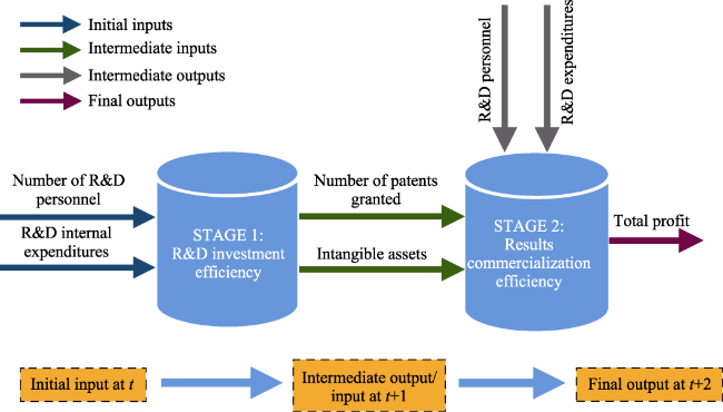
Fig. 2 Two-stage technological innovation efficiency (TIE) input-output evaluations |
Table 1 Definitions of the main variables |
| Variable nature | Variable name | Variable definitions | Provincial or enterprise level data | Symbolic representation |
|---|---|---|---|---|
| Dependent variable | Technological innovation efficiency of ISs | The comprehensive efficiency which is obtained by multiplying the stage efficiencies is the proxy variable of the technical efficiency. | Enterprise level | TIE |
| Core explanatory variable | Environmental regulation | The investment in the treatment of pollutants per unit, i.e., the intensity of environmental regulation | Provincial level | ER |
| Moderator variable | Financing constraints | Financing Constrained SA Index | Enterprise level | SA |
| Firm competitiveness | The proportion of the firm’s operating income to the total industry revenue, i.e., the market share | Enterprise level | MS | |
| Control variable | R&D investment scale | R&D investment as a percentage of operating income for the year | Enterprise level | R&D |
| Assets and liabilities ratio | Total corporate liabilities as a percentage of total corporate assets | Enterprise level | lnDAR | |
| Technical market turnover | Technology market turnover by province | Provincial level | lnTM | |
| Financial technology level | The comprehensive score of science and technology finance in each province as calculated via the entropy weight method② | Provincial level | TF | |
| Regional economic growth level | Regional GDP for the year | Provincial level | lnGDP |
② The entropy weight method is used to determine the weights of the four indicators: urban science and technology employment, urban financial practitioners, local financial science and technology expenditure, and the balance of the RMB loans of financial institutions in each province. |
Table 2 Descriptive statistics of the main variables |
| Variables | Observations | Mean | SD | Min | Q(0.25) | Median | Q(0.75) | Max | P value of the K-S normality test | P value of the S-W normality test |
|---|---|---|---|---|---|---|---|---|---|---|
| TIE | 165 | 0.1533 | 0.2017 | 0.0055 | 0.0279 | 0.0549 | 0.2108 | 0.9869 | <0.001 | <0.001 |
| ER | 165 | 0.8269 | 1.0592 | 0.1152 | 0.2751 | 0.4984 | 1.0836 | 8.1899 | <0.001 | <0.001 |
| SA | 165 | 6.8597 | 1.6527 | 3.4435 | 5.5747 | 6.9203 | 8.0490 | 10.6428 | 0.200 | 0.022 |
| MS | 165 | 0.5601 | 0.7145 | 0.0040 | 0.1168 | 0.3366 | 0.7494 | 4.5317 | <0.001 | <0.001 |
| R&D | 165 | 2.2858 | 1.4414 | 0.0400 | 1.1300 | 2.3800 | 3.4300 | 5.7600 | 0.001 | <0.001 |
| lnDAR | 165 | 3.8932 | 0.4707 | 2.4060 | 3.5482 | 4.0445 | 4.2650 | 4.7165 | <0.001 | <0.001 |
| lnTM | 165 | 5.2384 | 1.4396 | 1.1086 | 4.3580 | 5.5309 | 6.3507 | 8.3933 | 0.001 | 0.001 |
| TF | 165 | 0.2286 | 0.1373 | 0.0569 | 0.1222 | 0.1831 | 0.3373 | 0.5950 | <0.001 | <0.001 |
| lnGDP | 165 | 10.3377 | 0.6176 | 8.8233 | 9.9924 | 10.3339 | 10.7391 | 11.4261 | <0.001 | <0.001 |
Note: The prefix “ln” before the explanatory variables denotes that it takes the logarithmic form. Both the Kolmogorov-Smirnov (K-S) test and Shapiro-Wilk (S-W) test are normality tests used to test whether each main variable has a normal distribution. |
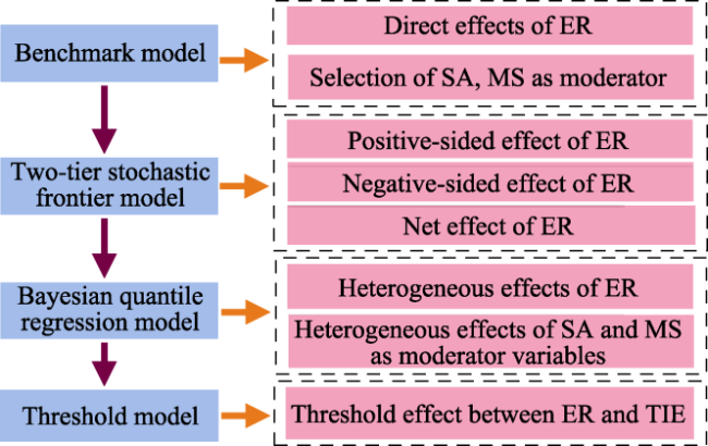
Fig. 3 Empirical framework of this study |
Table 3 Results of the benchmark model and moderator selection |
| Model variables | FE | RE | Two-step SYS-GMM | OLS | OLS | OLS | OLS | OLS | VIF |
|---|---|---|---|---|---|---|---|---|---|
| TIE (1) | TIE (2) | TIE (3) | TIE (4) | TIE (5) | TIE (6) | TIE (7) | TIE (8) | - | |
| L.TIE | - | - | 0.0054 | - | - | - | - | - | - |
| - | - | (0.13) | - | - | - | - | - | - | |
| ER | 0.0196** | 0.0182* | 0.0199*** | -0.0094 | 0.0293** | -0.1963** | 0.0358** | -0.0435 | 2.36 |
| (2.25) | (1.91) | (3.21) | (-0.68) | (2.12) | (-2.39) | (2.10) | (-1.40) | - | |
| SA | - | - | - | - | -0.0407*** | -0.0588*** | - | - | 3.93 |
| - | - | - | - | (-4.29) | (-5.18) | - | - | - | |
| MS | - | - | - | - | - | - | -0.0588** | -0.1077*** | 4.02 |
| - | - | - | - | - | - | (-2.55) | (-3.89) | - | |
| R&D | -0.0427** | -0.0708*** | -0.0237* | -0.0975*** | -0.1034*** | -0.1020*** | -0.0987*** | -0.1034*** | 1.29 |
| (-2.07) | (-4.12) | (-1.69) | (-10.23) | (-11.30) | (-11.37) | (-10.52) | (-11.14) | - | |
| lnDAR | 0.0685 | 0.0014 | 0.1122*** | -0.0248 | 0.0558* | 0.0379 | 0.0003 | 0.0044 | 1.83 |
| (1.36) | (0.05) | (3.55) | (-0.87) | (1.70) | (1.15) | (0.01) | (0.15) | - | |
| lnTM | 0.0584* | 0.0468** | -0.0304 | 0.0389*** | 0.0520*** | 0.0364*** | 0.0487*** | 0.0433*** | 2.61 |
| (1.88) | (2.45) | (-1.61) | (2.94) | (4.03) | (2.63) | (3.59) | (3.25) | - | |
| TF | -1.9504** | -0.5489*** | -0.3151 | -0.2256 | -0.3286* | -0.0740 | -0.3480* | -0.1093 | 5.35 |
| (-2.37) | (-2.60) | (-1.38) | (-1.13) | (-1.71) | (-0.35) | (-1.72) | (-0.51) | - | |
| lnGDP | 0.3911 | 0.0575 | 0.5158*** | -0.0359 | 0.0268 | 0.0317 | 0.0358** | 0.0327 | 2.86 |
| (0.82) | (1.30) | (3.49) | (-1.07) | (0.84) | (1.01) | (1.09) | (1.02) | - | |
| ER×SA | - | - | - | - | - | 0.0225*** | - | - | - |
| - | - | - | - | - | (2.79) | - | - | - | |
| ER×MS | - | - | - | - | - | - | - | 0.0266*** | - |
| - | - | - | - | - | - | - | (3.01) | - | |
| Constant | -3.9394 | -0.4100 | -5.3571*** | -0.0583 | -0.0467 | 0.1685 | -0.1643 | -0.0945 | - |
| (-0.80) | (-0.99) | (-3.49) | (-0.17) | (-0.14) | (0.50) | (-0.47) | (-0.28) | - | |
| R2 | 0.2816 | 0.2274 | - | 0.4133 | 0.4747 | 0.4996 | 0.4367 | 0.4677 | - |
| Hausman- χ2 test | chi2(6) = 17.62*** | - | - | - | - | - | - | - | |
| [P = 0.0073] | - | - | - | - | - | - | - | ||
| Sargan test | - | - | chi2(9) = 13.1935 | - | - | - | - | - | - |
| - | - | [P = 0.1540] | - | - | - | - | - | - | |
| N | 165 | 165 | 132 | 165 | 165 | 165 | 165 | 165 | 165 |
Note: The prefix “ln” before the explanatory variables denotes that it takes the logarithmic form. ***, **, and * indicate significance at the 1%, 5%, and 10% levels, respectively. The figures displayed in () are the posterior standard errors of the coefficients, and those displayed in [] are the P values of the corresponding test statistics. L.TIE indicates the one-period lag of the dependent variable. Column (4) presents the estimated result using pooled OLS. Columns (5)-(6) represent the estimation of the main effect of environmental regulation and the estimation of the moderating effect after incorporating the interaction term.Columns (7)-(8) present the estimates of the moderating effect of firm competitiveness after incorporating the interaction term. |
Table 4 Variance decomposition of the two-sided effects |
| Variance decomposition | Definition | Mathematical name | ER decomposition results |
|---|---|---|---|
| The two-sided effects | Promotion effect | 0.1401 | |
| Inhibition effect | 0.0344 | ||
| Random error | 0.0100 | ||
| Variance decomposition | Total variance of random error | 0.0209 | |
| The proportion of the two-sided effects | 0.9952 | ||
| The proportion of the inhibition effect | 0.0569 | ||
| The proportion of the promotion effect | 0.9431 |
Table 5 Proportion and quantile distributions of the effects |
| Core explanatory variable | Effects | Number | Mean | SD | Min | Q(0.25) | Median | Q(0.75) | Max |
|---|---|---|---|---|---|---|---|---|---|
| ER | Promotion effect | 165 | 14.01 | 15.28 | 2.76 | 3.82 | 8.51 | 17.98 | 81.88 |
| Inhibition effect | 165 | 3.44 | 1.89 | 2.76 | 2.76 | 2.76 | 2.83 | 14.08 | |
| Net effect | 165 | 10.57 | 15.89 | -11.31 | 0.99 | 5.75 | 15.22 | 79.12 |
Note: % refers to taking the percentiles of mean, SD, and Q. The same below. |
Table 6 Annual variation characteristics of the two-sided effects of ER on TIE |
| Year | Effects | Number | Mean | SD |
|---|---|---|---|---|
| 2017 | Promotion effect | 33 | 13.17 | 14.37 |
| Inhibition effect | 33 | 5.73 | 3.66 | |
| Net effect | 33 | 7.44 | 15.90 | |
| 2018 | Promotion effect | 33 | 10.60 | 11.50 |
| Inhibition effect | 33 | 5.99 | 4.07 | |
| Net effect | 33 | 4.61 | 13.37 | |
| 2019 | Promotion effect | 33 | 7.04 | 6.11 |
| Inhibition effect | 33 | 8.77 | 7.60 | |
| Net effect | 33 | -1.73 | 11.24 | |
| 2020 | Promotion effect | 33 | 13.06 | 12.33 |
| Inhibition effect | 33 | 1.00 | 0.19 | |
| Net effect | 33 | 12.06 | 12.39 | |
| 2021 | Promotion effect | 33 | 14.48 | 18.38 |
| Inhibition effect | 33 | 4.99 | 3.16 | |
| Net effect | 33 | 9.49 | 19.40 |
Table 7 Variation characteristics of the two-sided effects of ER on TIE by different regions |
| Different regions | Effects | Number | Mean | SD |
|---|---|---|---|---|
| Enterprises in coastal provinces | Promotion effect | 95 | 14.42 | 14.04 |
| Inhibition effect | 95 | 2.65 | 1.42 | |
| Net effect | 95 | 11.77 | 14.46 | |
| Enterprises in inland provinces | Promotion effect | 70 | 14.67 | 16.85 |
| Inhibition effect | 70 | 3.89 | 2.16 | |
| Net effect | 70 | 10.78 | 17.54 | |
| Enterprises in eastern provinces | Promotion effect | 95 | 12.89 | 14.03 |
| Inhibition effect | 95 | 3.50 | 2.04 | |
| Net effect | 95 | 9.39 | 14.71 | |
| Enterprises in central provinces | Promotion effect | 30 | 15.71 | 16.27 |
| Inhibition effect | 30 | 4.67 | 0.12 | |
| Net effect | 30 | 11.04 | 16.32 | |
| Enterprises in western provinces | Promotion effect | 40 | 12.44 | 12.24 |
| Inhibition effect | 40 | 1.80 | 0.20 | |
| Net effect | 40 | 10.64 | 12.31 |
Table 8 Variation characteristics of the two-sided effects of ER on TIE based on property rights |
| Property right nature | Effects | Number | Mean | SD |
|---|---|---|---|---|
| State-owned enterprises | Promotion effect | 115 | 13.10 | 14.68 |
| Inhibition effect | 115 | 1.49 | 0.37 | |
| Net effect | 115 | 11.61 | 14.79 | |
| Nonstate-owned enterprises | Promotion effect | 50 | 12.74 | 12.74 |
| Inhibition effect | 50 | 1.00 | 0.11 | |
| Net effect | 50 | 11.74 | 12.79 |
Table 9 Bayesian quantile estimates of ER and the moderating effects of SA |
| Model variables | (9) | (10) | (11) | (12) | (13) | (14) | (15) | (16) | (17) | (18) |
|---|---|---|---|---|---|---|---|---|---|---|
| TIE-Q(0.05) | TIE-Q(0.25) | TIE-Q(0.50) | TIE-Q(0.75) | TIE-Q(0.95) | TIE-Q(0.05) | TIE-Q(0.25) | TIE-Q(0.50) | TIE-Q(0.75) | TIE-Q(0.95) | |
| ER | 0.0156** | 0.0144* | 0.0228* | 0.0287* | 0.0504*** | -0.0433 | -0.0910** | -0.1637*** | -0.2365*** | -0.2620*** |
| (0.0001) | (0.0001) | (0.0001) | (0.0002) | (0.0002) | (0.0003) | (0.0004) | (0.0006) | (0.0007) | (0.0009) | |
| SA | 0.0008 | -0.0055 | -0.0277*** | -0.0475*** | -0.0779*** | -0.0062 | -0.0156*** | -0.0421*** | -0.0704*** | -0.1060*** |
| (0.0000) | (0.0000) | (0.0001) | (0.0001) | (0.0002) | (0.0000) | (0.0001) | (0.0001) | (0.0001) | (0.0002) | |
| R&D | -0.0136*** | -0.0377*** | -0.0844*** | -0.1090*** | -0.1355*** | -0.0121*** | -0.0363*** | -0.0772*** | -0.1034*** | -0.1396*** |
| (0.0000) | (0.0001) | (0.0001) | (0.0001) | (0.0001) | (0.0000) | (0.0001) | (0.0001) | (0.0001) | (0.0001) | |
| lnDAR | 0.0005 | 0.0104 | 0.0393* | 0.0891*** | 0.1712*** | -0.0024 | -0.0026 | 0.0187 | 0.0686** | 0.1561*** |
| (0.0001) | (0.0001) | (0.0002) | (0.0003) | (0.0006) | (0.0001) | (0.0001) | (0.0002) | (0.0003) | (0.0005) | |
| lnTM | 0.0047 | 0.0098* | 0.0433*** | 0.0685*** | 0.0989*** | -0.0026 | 0.0015 | 0.0212 | 0.0434*** | 0.0800*** |
| (0.0000) | (0.0001) | (0.0001) | (0.0001) | (0.0002) | (0.0000) | (0.0001) | (0.0001) | (0.0001) | (0.0002) | |
| TF | 0.0125 | 0.0289 | -0.3849** | -0.3373* | -0.0318 | 0.0962 | 0.1393 | -0.0954 | -0.1132 | 0.4022 |
| (0.0005) | (0.0010) | (0.0019) | (0.0020) | (0.0028) | (0.0006) | (0.0010) | (0.0021) | (0.0021) | (0.0029) | |
| lnGDP | -0.0005 | 0.0024 | 0.0462 | 0.0011 | -0.1656*** | -0.0053 | -0.0006 | 0.0384 | 0.0253 | -0.2075*** |
| (0.0001) | (0.0002) | (0.0003) | (0.0003) | (0.0006) | (0.0001) | (0.0002) | (0.0003) | (0.0003) | (0.0005) | |
| ER*SA | - | - | - | - | - | 0.0060** | 0.0111*** | 0.0193*** | 0.0286*** | 0.0305*** |
| - | - | - | - | - | (0.0000) | (0.0000) | (0.0001) | (0.0001) | (0.0001) | |
| Constant | 0.0067 | 0.0394 | -0.2817 | 0.1293 | 1.7505*** | 0.1457 | 0.2299 | 0.0483 | 0.2314 | 2.5217*** |
| (0.0009) | (0.0017) | (0.0030) | (0.0031) | (0.0068) | (0.0012) | (0.0018) | (0.0031) | (0.0028) | (0.0058) |
Note: The prefix “ln” before the explanatory variables denotes that it takes the logarithmic form. ***, **, and * indicate significance at the 1%, 5%, and 10% levels, respectively. The figures displayed in () are the posterior standard errors of the coefficients. (9)-(13) present the impact of environmental regulation on technical efficiency under financing constraints at all the observed quantiles. (14)-(18) add the interaction effects between environmental regulations and financing constraints. |
Table 10 Bayesian quantile estimates of ER and the moderating effects of MS |
| Model variables | (19) | (20) | (21) | (22) | (23) | (24) | (25) | (26) | (27) | (28) |
|---|---|---|---|---|---|---|---|---|---|---|
| TIE-Q(0.05) | TIE-Q(0.25) | TIE-Q(0.50) | TIE-Q(0.75) | TIE-Q(0.95) | TIE-Q(0.05) | TIE-Q(0.25) | TIE-Q(0.50) | TIE-Q(0.75) | TIE-Q(0.95) | |
| ER | 0.0153** | 0.0142 | 0.0230 | 0.0364** | 0.0604*** | 0.0022 | -0.0099 | -0.0287 | -0.0713*** | -0.0632** |
| (0.0001) | (0.0001) | (0.0001) | (0.0002) | (0.0002) | (0.0001) | (0.0002) | (0.0002) | (0.0003) | (0.0003) | |
| MS | 0.0003 | -0.0047 | -0.0272 | -0.0708*** | -0.0913*** | -0.0085 | -0.0258 | -0.0577** | -0.1173*** | -0.1624*** |
| (0.0001) | (0.0001) | (0.0002) | (0.0002) | (0.0001) | (0.0001) | (0.0002) | (0.0003) | (0.0002) | (0.0003) | |
| R&D | -0.0136*** | -0.0346*** | -0.0716*** | -0.1041*** | -0.1423*** | -0.0131*** | -0.0373*** | -0.0725*** | -0.1086*** | -0.1410 |
| (0.0000) | (0.0001) | (0.0001) | (0.0001) | (0.0004) | (0.0000) | (0.0001) | (0.0001) | (0.0001) | (0.0001) | |
| lnDAR | 0.0023 | 0.0022 | 0.0036 | 0.0128 | 0.0443 | 0.0006 | -0.0015 | 0.0001 | 0.0037 | 0.0477 |
| (0.0001) | (0.0001) | (0.0002) | (0.0003) | (0.0002) | (0.0001) | (0.0001) | (0.0002) | (0.0003) | (0.0003) | |
| lnTM | 0.0043 | 0.0092 | 0.0337 | 0.0640*** | 0.0966*** | 0.0012 | 0.0068 | 0.0285** | 0.0509*** | 0.0910*** |
| (0.0000) | (0.0001) | (0.0001) | (0.0001) | (0.0002) | (0.0000) | (0.0001) | (0.0001) | (0.0001) | (0.0002) | |
| TF | 0.0173 | 0.0453 | -0.2536 | -0.3450* | -0.3626 | 0.0607 | 0.1108 | -0.1125 | -0.1133 | 0.1075 |
| (0.0005) | (0.0010) | (0.0017 | (0.0020) | (0.0032) | (0.0006) | (0.0011) | (0.0019) | (0.0019) | (0.0026) | |
| lnGDP | -0.0013 | 0.0015 | 0.0367 | 0.0041 | -0.0992 | -0.0044 | -0.0022 | 0.0341 | 0.0271 | -0.1581*** |
| (0.0001) | (0.0002) | (0.0003) | (0.0003) | (0.0007) | (0.0001) | (0.0002) | (0.0003) | (0.0003) | (0.0005) | |
| ER*MS | - | - | - | - | - | 0.0042 | 0.0095* | 0.0211** | 0.0392*** | 0.0420*** |
| - | - | - | - | - | (0.0000) | (0.0001) | (0.0001) | (0.0001) | (0.0001) | |
| Constant | 0.0147 | 0.0369 | -0.2399 | 0.1167 | 0.0604 | 0.0706 | 0.1195 | -0.1561 | 0.0251 | 1.7959*** |
| (0.0009) | (0.0017) | (0.0029) | (0.0035) | (0.0078) | (0.0010) | (0.0018) | (0.0030) | (0.0031) | (0.0059) |
Note: The prefix “ln” before the explanatory variables denotes that it takes the logarithmic form. ***, **, and * indicate significance at the 1%, 5%, and 10% levels, respectively. The figures displayed in () are the posterior standard errors of the coefficients. (19)-(23) present the impact of environmental regulation on technical efficiency under firm competitiveness at all the observed quantiles. (24)-(28) add the interaction effects between environmental regulations and firm competitiveness. |
Table 11 Threshold effects test |
| Threshold variable | Regime variable | Threshold type | BS | F statistics | P value | The existence of the threshold | Threshold value | 95% threshold confidence interval | |
|---|---|---|---|---|---|---|---|---|---|
| Lower | Higher | ||||||||
| SA | Single | 300 | 14.40 | 0.0933 | Yes | 8.4537 | 8.4231 | 8.6278 | |
| ER | Double | 300 | 25.17 | 0.0133 | Yes | 7.8473 | 7.6620 | 7.9461 | |
| Triple | 300 | 8.61 | 0.8367 | No | 5.7277 | 5.6341 | 5.8174 | ||
| MS | Single | 300 | 25.55 | 0.0067 | Yes | 0.3336 | 0.3172 | 0.3478 | |
| ER | Double | 300 | 11.96 | 0.0800 | Yes | 0.2595 | 0.2333 | 0.2832 | |
| Triple | 300 | 9.44 | 0.1333 | No | 0.1869 | 0.1732 | 0.1923 | ||
Note: The regime variable is the core explanatory variable that is affected by the threshold variable. BS represents the number of times to bootstrap. |
Table 12 Results of the double threshold regression |
| Variables | (29) | Variables | (30) |
|---|---|---|---|
| ER (SA≤7.8473) | 0.0151 | ER (MS≤0.2595) | 0.0829** |
| (0.33) | (1.97) | ||
| ER (7.8473<SA<8.4537) | 0.3275*** | ER (0.2595<MS<0.3336) | 0.2567*** |
| (5.83) | (5.52) | ||
| ER (SA≥8.4537) | 0.0159 | ER (MS≥0.3336) | 0.0121 |
| (1.10) | (0.85) | ||
| R&D | -0.0336*** | R&D | -0.0382*** |
| (-2.78) | (-3.14) | ||
| lnDAR | 0.0360 | lnDAR | 0.0423 |
| (0.78) | (0.91) | ||
| lnTM | 0.0397 | lnTM | 0.0543* |
| (1.37) | (1.88) | ||
| TF | -1.0471** | TF | -0.9427* |
| (-2.12) | (-1.87) | ||
| lnGDP | 0.4311** | lnGDP | 0.4104* |
| (1.96) | (1.83) | ||
| Constant | -4.3792** | Constant | -4.2785* |
| (-1.96) | (-1.88) | ||
| R2 | 0.3568 | R2 | 0.3490 |
Note: The prefix “ln” before the explanatory variables denotes that it takes the logarithmic form. ***, **, and * indicate significance at the 1%, 5%, and 10% levels, respectively. The figures displayed in () are the t values of the coefficients. |
Table 13 The specific number of enterprises and years in different threshold intervals |
| Threshold interval | Enterprises stock code | Sum |
|---|---|---|
| SA≤7.8473 | 002756(5), 002478(5), 002443(5), 002318(5), 002110(5), 002075(5), 000923(5), 000778(5), 603878(5), 601005(5), 601003(5), 600581(5), 600569(5), 600516(5), 600507(5), 600399(5), 600307(5), 600295(5), 600282(5), 600231(5), 600126(5), 000708(4), 000629(4), 000761(1) | 114 |
| 7.8473<SA<8.4537 | 600808(5), 000932(5), 000825(5), 600022(5), 000761(4), 000959(1), 000708(1), 000629(1) | 27 |
| SA≥8.4537 | 600019(5), 000709(5), 600010(5), 000898(5), 000959(4) | 24 |
| MS≤0.2595 | 002756(5), 002478(5), 002443(5), 002318(5), 000923(5), 000629(5), 603978(5), 600516(5), 600507(5), 600399(5), 002075(4), 000708(4), 601005(3), 600581(3), 002110(2), 600231(2), 600295(1), 600126(1) | 71 |
| 0.2595<MS<0.3336 | 600231(3), 600581(2), 600295(2), 000959(1), 600569(1), 600126(1) | 10 |
| MS≥0.3336 | 000932(5), 000898(5), 000825(5), 000778(5), 000761(5), 000709(5), 601003(5), 000761(5), 000709(5), 601003(5), 600808(5), 600307(5), 600282(5), 600022(5), 600019(5), 600010(5), 600569(4), 002110(3), 000959(3), 600126(3), 601005(2), 600295(2), 000708(1) | 84 |
Note: The enterprise name is replaced by a stock code. The figures displayed in () are the number of years for the enterprise in each threshold interval. |
| [1] |
|
| [2] |
|
| [3] |
|
| [4] |
|
| [5] |
|
| [6] |
|
| [7] |
|
| [8] |
|
| [9] |
|
| [10] |
|
| [11] |
|
| [12] |
|
| [13] |
|
| [14] |
|
| [15] |
|
| [16] |
|
| [17] |
|
| [18] |
|
| [19] |
|
| [20] |
|
| [21] |
|
| [22] |
|
| [23] |
|
| [24] |
|
| [25] |
|
| [26] |
|
| [27] |
|
| [28] |
|
| [29] |
|
| [30] |
|
| [31] |
|
| [32] |
|
| [33] |
|
| [34] |
|
| [35] |
|
| [36] |
|
| [37] |
|
| [38] |
|
| [39] |
|
| [40] |
|
| [41] |
|
| [42] |
|
| [43] |
|
| [44] |
|
| [45] |
|
| [46] |
|
| [47] |
|
| [48] |
|
| [49] |
|
| [50] |
|
| [51] |
|
| [52] |
|
| [53] |
|
| [54] |
|
| [55] |
|
| [56] |
|
| [57] |
|
| [58] |
|
| [59] |
|
| [60] |
|
| [61] |
|
/
| 〈 |
|
〉 |