
Journal of Resources and Ecology >
Industrial Carbon Reduction Potential Measurement and Scenario Prediction in Shaanxi Province
|
WANG Wenjun, E-mail: wwjunxida@snnu.edu.cn |
Received date: 2023-03-20
Accepted date: 2023-09-25
Online published: 2024-07-25
Supported by
The Shaanxi Social Science Federation Foundation Project(2021HZ1118)
The Shaanxi Normal University Graduate Student Innovation Team Project(TD2020006Y)
Promoting industrial carbon reduction is an inevitable step for achieving the Chinese carbon peak and neutrality targets. Based on the industrial energy consumption data of Shaanxi Province from 2011 to 2020, this study uses the IPCC calculation method to calculate the industrial carbon emissions in Shaanxi Province. The prediction model for industrial carbon emissions in Shaanxi Province was constructed based on the STIRPAT model from three aspects: population, economy, and technology. By setting three scenario models, the industrial carbon emissions from 2021 to 2035 and the time to achieve peak carbon neutrality were then predicted. The results show that the industry in Shaanxi Province cannot achieve a carbon peak under the baseline scenario, although it can achieve carbon peaking in 2030 under a low-carbon scenario or in 2025 under an enhanced low-carbon scenario. The predicted carbon peak values are 209.11 million t and 188.36 million t, respectively. Based on the results of this study, four policy recommendations are proposed: (1) strengthen publicity and education efforts to increase public participation in energy conservation and emission reduction; (2) promote the green transformation of industry and develop a green economy, including the active development of energy-saving and emission reduction technologies; (3) accelerate the implementation of industrial carbon reduction; and (4) promote the development and utilization of clean energy and increase efforts to adjust the energy structure.
WANG Wenjun , YING Xinru , KOU Chenlu . Industrial Carbon Reduction Potential Measurement and Scenario Prediction in Shaanxi Province[J]. Journal of Resources and Ecology, 2024 , 15(4) : 860 -869 . DOI: 10.5814/j.issn.1674-764x.2024.04.007
Table 1 Industrial carbon emission forecasting model index system for Shaanxi Province |
| Model | First level indicator | Second level indicator | Unit | Symbol | Properties |
|---|---|---|---|---|---|
| Industrial carbon emission projections | Population | Year-end population | 104 persons | P1 | + |
| Economy | GDP | 108 yuan | A1 | + | |
| Industrial value added per capita | 104 yuan person-1 | A2 | + | ||
| Technology | Industrial carbon emission intensity | t CO2 (104 yuan)-1 | T1 | - | |
| Industrial energy intensity | t standard coal (104 yuan)-1 | T2 | - |
Table 2 Correlation coefficients of industrial carbon emissions and various influencing factors for the time-period of 2010 to 2020 |
| Influencing factors | Year-end population | GDP | Industrial value added per capital | Industrial carbon emission intensity | Industrial energy intensity |
|---|---|---|---|---|---|
| Industrial carbon emissions | 0.793 | 0.879 | 0.806 | -0.005 | -0.779 |
Table 3 Energy conversion factors of standard coal |
| Types of energy | Raw coal | Coke | Gas | Crude oil | Gasoline | Kerosene | Diesel |
|---|---|---|---|---|---|---|---|
| Discount factor for standard coal (kgce kg-1) | 0.7143 | 0.9714 | 1.33 | 1.4286 | 1.4714 | 1.4714 | 1.4571 |
Table 4 Specific data for the factors influencing industrial carbon emissions in Shaanxi Province in 2011-2020 |
| Year | lnY | lnP1 | lnA1 | lnA2 | lnT1 | lnT2 |
|---|---|---|---|---|---|---|
| 2011 | 9.25 | 8.23 | 9.41 | 3.56 | -0.15 | -0.29 |
| 2012 | 9.41 | 8.23 | 9.56 | 3.67 | -0.14 | -0.36 |
| 2013 | 9.59 | 8.23 | 9.67 | 3.82 | -0.08 | -0.40 |
| 2014 | 9.65 | 8.24 | 9.76 | 3.90 | -0.11 | -0.44 |
| 2015 | 9.84 | 8.24 | 9.79 | 3.81 | 0.04 | -0.42 |
| 2016 | 9.84 | 8.25 | 9.85 | 3.84 | -0.02 | -0.45 |
| 2017 | 9.85 | 8.25 | 9.97 | 3.98 | -0.13 | -0.54 |
| 2018 | 9.81 | 8.26 | 10.08 | 4.13 | -0.28 | -0.62 |
| 2019 | 9.84 | 8.26 | 10.16 | 4.12 | -0.32 | -0.65 |
| 2020 | 9.85 | 8.28 | 10.17 | 4.09 | -0.32 | -0.63 |
Table 5 Ordinary least squares estimation results |
| Variable | Coefficient | Standard error | Standard coefficient | t | P | VIF |
|---|---|---|---|---|---|---|
| $\ln \alpha $ | -5.218 | 1.709 | -3.053 | 0.055 | ||
| $\ln {{P}_{1}}$ | 0.875 | 0.243 | 0.049 | 3.602 | 0.037 | 15.958 |
| $\ln {{A}_{1}}$ | 0.774 | 0.081 | 0.848 | 9.500 | 0.002 | 699.187 |
| $\ln {{A}_{2}}$ | 0.006 | 0.025 | 0.005 | 0.224 | 0.837 | 41.032 |
| $\ln {{T}_{1}}$ | 1.168 | 0.041 | 0.601 | 28.702 | <0.001 | 38.456 |
| $\ln {{T}_{2}}$ | -0.500 | 0.195 | -0.269 | -2.557 | 0.083 | 970.825 |
Note: Adjusted R2=1, F-statistic=17562.966, P (F-statistic) < 0.001. |
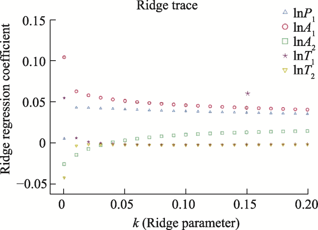
Fig. 1 Ridge trace plot, where the range of k is 0-1, the horizontal scale is 0.2, and the vertical scale is 0.2 |
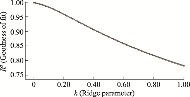
Fig. 2 R2-k diagram, where the range of k is 0-1, the horizontal scale is 0.2, and the vertical scale is 0.05 |
Fig. 3 Ridge trace plot, where the range of k is 0-0.2, the horizontal scale and the vertical scale both are 0.05 |
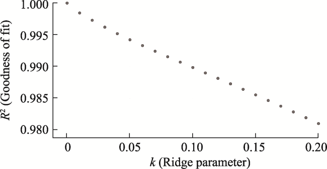
Fig. 4 R2-k diagram, where the range of k is 0-0.2, the horizontal scale is 0.05, and the vertical scale is 0.005 |
Table 6 Ridge regression results |
| Variable | Coefficient | Standard error | Standard coefficient | t | P |
|---|---|---|---|---|---|
| lnP1 | 3.629 | 1.345 | 0.202 | 2.698 | 0.074 |
| lnA1 | 0.414 | 0.044 | 0.454 | 9.418 | 0.002 |
| lnA2 | 0.265 | 0.084 | 0.227 | 3.155 | 0.051 |
| lnT1 | 1.148 | 0.088 | 0.590 | 13.096 | <0.001 |
| lnT2 | -0.511 | 0.074 | -0.275 | -6.898 | 0.006 |
| Constant | -25.412 | 10.796 | <0.001 | -2.354 | 0.099 |
Note: R2=0.9948, F-statistic=116.558, P (F-statistic)=0.0012. |
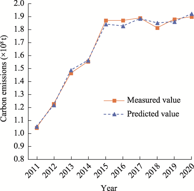
Fig. 5 Fitting of the actual and predicted values of industrial carbon emissions from 2011 to 2020 |
Table 7 Model predictions fitted to the actual values |
| Year | Industrial carbon emissions (×104 t) | |||||||||
|---|---|---|---|---|---|---|---|---|---|---|
| 2011 | 2012 | 2013 | 2014 | 2015 | 2016 | 2017 | 2018 | 2019 | 2020 | |
| Measured value | 10445.27 | 12261.13 | 14655.74 | 15556.25 | 18684.84 | 18683.48 | 18882.13 | 18157.55 | 18788.96 | 19000.00 |
| Predicted value | 10517.87 | 12197.73 | 14852.77 | 15623.46 | 18407.47 | 18272.80 | 18822.90 | 18492.77 | 18626.25 | 19208.81 |
| Percentage of error | 0.70% | -0.52% | 1.34% | 0.43% | -1.48% | -2.20% | -0.31% | 1.85% | -0.87% | 1.10% |
Table 8 Parameter settings for the three scenarios |
| Scenario | Period | Annual average growth rate (%) | ||||
|---|---|---|---|---|---|---|
| P1 | A1 | A2 | T1 | T2 | ||
| Baseline scenario | 2021-2025 | 0.5 | 9 | 5 | -5 | -5 |
| 2026-2030 | 0.4 | 11 | 8 | -7 | -5.5 | |
| 2031-2035 | 0.3 | 12 | 11 | -9 | -6.5 | |
| Low-carbon scenario | 2021-2025 | 0.4 | 8 | 4 | -6 | -6 |
| 2026-2030 | 0.2 | 10 | 7 | -8 | -6.5 | |
| 2031-2035 | 0 | 11 | 10 | -10 | -7 | |
| Enhanced low-carbon scenario | 2021-2025 | 0.3 | 7 | 3 | -7 | -7 |
| 2026-2030 | 0 | 9.5 | 6 | -9 | -7.5 | |
| 2031-2035 | -0.1 | 10 | 9 | -11 | -8 | |
Table 9 Forecast of industrial carbon emissions from 2021- 2035 (unit: 104 t) |
| Year | Baseline scenario | Low-carbon scenario | Enhanced low-carbon scenario |
|---|---|---|---|
| 2021 | 19002.72 | 18883.53 | 18656.36 |
| 2022 | 19452.83 | 19215.42 | 18721.33 |
| 2023 | 19987.36 | 19573.44 | 18784.99 |
| 2024 | 20588.86 | 19742.59 | 18808.67 |
| 2025 | 21264.77 | 20079.34 | 18836.80 |
| 2026 | 21789.51 | 20279.39 | 18813.27 |
| 2027 | 22352.92 | 20434.88 | 18797.20 |
| 2028 | 23016.85 | 20596.09 | 18705.90 |
| 2029 | 23662.72 | 20774.12 | 18535.51 |
| 2030 | 24248.82 | 20911.24 | 18359.35 |
| 2031 | 24820.24 | 20873.42 | 18068.73 |
| 2032 | 25475.81 | 20713.28 | 17673.90 |
| 2033 | 26147.06 | 20443.01 | 17177.69 |
| 2034 | 26829.35 | 19958.36 | 16538.14 |
| 2035 | 27233.85 | 19790.82 | 15786.55 |
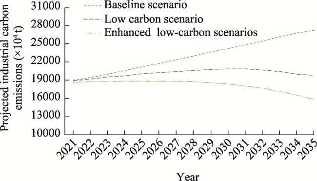
Fig. 6 Trends in Industrial carbon emissions from 2021 to 2035 under the three scenarios |
| [1] |
|
| [2] |
|
| [3] |
|
| [4] |
|
| [5] |
|
| [6] |
|
| [7] |
|
| [8] |
|
| [9] |
|
| [10] |
|
| [11] |
|
/
| 〈 |
|
〉 |
