
Journal of Resources and Ecology >
Application of Bilateral Gamma Distribution in Carbon Trading
Received date: 2022-07-13
Accepted date: 2023-06-05
Online published: 2024-03-14
Introducing carbon financial derivatives and improving the carbon trading system are indispensable means for promoting carbon emission reductions. However, the reasonable pricing of carbon financial derivatives is crucial for launching related financial products. Here, the bilateral gamma distribution was used to fit the carbon quota yield series for the first time and compute the volatility of the carbon quota price, based on which the carbon option price was calculated by optimizing the option pricing model. The experimental results show that the carbon quota yield sequence approximately follows the bilateral gamma distribution and the model is reasonable for carbon option pricing. Subsequently, considering the relationship between continuous rise and fall rate in yield and the influence of trading volume on price, the formula of conditional probability of price rise and fall is derived by using bilateral gamma distribution, and numerical verification is carried out. Therefore, bilateral gamma distribution can be used for option pricing and price probability inference in carbon trading.
DONG Hongling , HU Yue , FU Le , ZHAI Jiayang . Application of Bilateral Gamma Distribution in Carbon Trading[J]. Journal of Resources and Ecology, 2024 , 15(2) : 396 -403 . DOI: 10.5814/j.issn.1674-764x.2024.02.013
Table 1 Descriptive statistical analysis of yield sequence |
| Sequence | Min | Max | Average | SD | SK | K |
|---|---|---|---|---|---|---|
| Yield | -10.70 | 6.19 | 0.1 386 | 1.4 393 | -1.582 | 13.602 |
Note: SD: Standard Deviation; SK: Skewness (Numerical characteristics of the degree of asymmetry in statistical data distribution); K: Kurtosis (The number of features that characterizes the peak of the probability density distribution curve at the average value). |
Table 2 Parameter estimates |
| Situation | Fitting parameters | P-value (1) | Adjust parameters | P-value (2) |
|---|---|---|---|---|
| Continuous rise | 0.245 | 0.5128 | ||
| Continuous decline | 0.419 | 0.9379 |
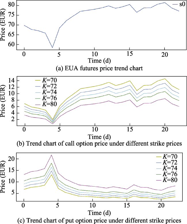
Fig. 1 Trend of underlying asset and option prices |
Table 3 Conditional probability of future price decline |
| Continuous rise yield, continuous fall yield (a, b) | Turnover v (k) | ||||
|---|---|---|---|---|---|
| 10 | 30 | 50 | 80 | 100 | |
| (0.005, 0.01) | 0.059 | 0.279 | 0.640 | 0.664 | 0.891 |
| (0.01, 0.01) | 0.062 | 0.142 | 0.327 | 0.486 | 0.652 |
| (0.05, 0.01) | 0.066 | 0.031 | 0.258 | 0.339 | 0.456 |
| (0.08, 0.01) | 0.072 | 0.019 | 0.163 | 0.221 | 0.288 |
| (0.1, 0.01) | 0.077 | 0.015 | 0.062 | 0.178 | 0.231 |
| (0.1, 0.03) | 0.081 | 0.148 | 0.171 | 0.229 | 0.465 |
| (0.1, 0.05) | 0.112 | 0.162 | 0.463 | 0.396 | 0.649 |
| (0.1, 0.1) | 0.129 | 0.239 | 0.541 | 0.463 | 0.731 |
| [1] |
|
| [2] |
|
| [3] |
|
| [4] |
|
| [5] |
|
| [6] |
|
| [7] |
|
| [8] |
|
| [9] |
|
| [10] |
|
| [11] |
|
| [12] |
|
| [13] |
|
| [14] |
|
| [15] |
|
| [16] |
|
| [17] |
|
| [18] |
|
| [19] |
|
| [20] |
|
| [21] |
|
| [22] |
|
| [23] |
|
| [24] |
|
| [25] |
|
| [26] |
|
| [27] |
|
| [28] |
|
| [29] |
|
| [30] |
|
| [31] |
|
/
| 〈 |
|
〉 |