Urban-Rural Integration and Green Development

The Spatial Impact of the Accessibility of Urban Green Infrastructure on Housing Prices in Nanjing, China

  • GAO Zhoubing , 1, 2 ,
  • ZHU Junjun 1, 2 ,
  • LV Ligang , 1, 2, * ,
  • LI Yongle 1 ,
  • WANG Junxiao 1
Expand
  • 1. School of Public Administration, Nanjing University of Finance and Economics, Nanjing 210023, China
  • 2. Key Laboratory of Coastal Zone Development and Protection, Ministry of Natural Resources, Nanjing 210000, China
*LV Ligang, E-mail:

GAO Zhoubing, E-mail:

Received date: 2022-09-02

  Accepted date: 2023-05-02

  Online published: 2024-03-14

Supported by

The National Natural Science Foundation of China(41801169)

The Open Fund Project of Key Laboratory of Coastal Zone Development and Protection, Ministry of Natural Resources(2019CZEPK06)

Abstract

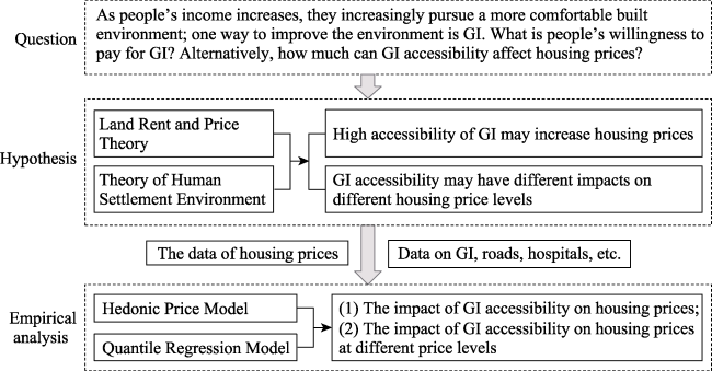
The reasonable allocation of green infrastructure (GI) can improve the environmental quality of human settlements and urban residents’ happiness. We used hedonic price and quantile regression models to quantitatively examine the impact of GI accessibility on housing prices, and the heterogeneity of this impact across different housing prices. The results showed that: (1) GI accessibility significantly affected housing prices. In addition, every 1% increase in GI area increased housing prices by approximately 0.3%. (2) GI accessibility had different effects on different housing prices; that is, different housing prices had different sensitivities to GI accessibility. This was especially true in the 25%-75% range of housing prices, where housing prices were negatively correlated with the time to the nearest GI. During urban development, reasonable planning and construction of urban GI should be undertaken to meet urban residents’ needs for GI and promote sustainable urban development.

Cite this article

GAO Zhoubing , ZHU Junjun , LV Ligang , LI Yongle , WANG Junxiao . The Spatial Impact of the Accessibility of Urban Green Infrastructure on Housing Prices in Nanjing, China[J]. Journal of Resources and Ecology, 2024 , 15(2) : 329 -337 . DOI: 10.5814/j.issn.1674-764x.2024.02.008

1 Introduction

Green infrastructure (GI), as an ecological barrier, is important for improving the environmental quality of human settlements and maintaining urban sustainable development (Li et al., 2021). GI refers to an interconnected, organic, and unified network system of green spaces comprising various open spaces and natural areas, including greenways, wetlands, rain gardens, and vernacular vegetation (Conway et al., 2020; Hoover, et al., 2020; Li et al., 2021). It can help in managing stormwater, improving water quality, and reducing the urban heat island effect (Suppakittpaisarn et al., 2019; Hoover, et al., 2020). The core idea is to use soil and/or vegetation characteristics to improve the retention capacity of water or sewage sheds, and use the natural process of water circulation to manage rainwater (Berland et al., 2017). In recent years, green development and infrastructure construction have received increasing attention from the state. For example, an important recommendation in the “Proposal of the CPC Central Committee on Formulating the Fourteenth Five Year Plan for National Economic and Social Development and the Vision for the Year 2035”, released in 2020, was “Building a modern infrastructure system that is complete, efficient, practical, intelligent, green, safe and reliable” (Wang and Qin, 2021).
In recent years, numerous studies have examined the impact of GI on housing prices using the hedonic price model (Nazir et al., 2015; Hoover et al., 2020; Sohn et al., 2020; Dell’Anna et al., 2022). A study on Shanghai showed that there was a significant negative correlation between housing prices and the time to the nearest green space, that is, the shorter the time to the nearest green space, the higher the housing prices (Yin et al., 2009). A similar finding was observed for Urumqi, whereby as the distance to the park green space increased by 1 km, the average housing prices decreased by approximately 20000 yuan (Liu and Chen, 2020). Another study in Germany showed that the size of the urban green space has a greater impact on housing prices than that of the distance to the green space (Liebelt et al., 2018). However, a study in Omaha found no significant effect of GI on housing prices within different buffer distances (Hoover et al., 2020). Given the differing impacts across contexts, the impact of GI on housing prices needs further investigation.
As a megacity in eastern China and the gateway city of the Yangtze River Economic Belt, Nanjing has a good natural resource base (Gao et al., 2022). However, an analysis of the Nanjing Ecological Civilization Construction Plan 2018-2020 suggests that as Nanjing is rapidly urbanizing and its economy is developing, the resource constraints are tightening, and the environmental quality of human settlements is deteriorating (Gao et al., 2022). Therefore, taking Nanjing as an example, to explore the impact of GI accessibility on housing prices, which has important practical significance for promoting the rational allocation of GI and improving the environmental quality of human settlements, and can also provide a reference for the sustainable development of other cities. To sum up, we collected 89898 second-hand housing prices and housing characteristics in 4357 communities in Nanjing in February 2021. The hedonic price model was first used to explore the direction and magnitude of the impact of GI accessibility on housing prices. Then, the quantile regression model was used to study the heterogeneous impacts of GI accessibility on different housing prices.

2 Study area and research framework

2.1 Study area

Nanjing, located in the middle of the lower reaches of the Yangtze River, is an important central city in eastern China. By the end of 2021, the city’s total area of 6587.04 km2 housed 9.4234 million permanent population, with a green cover area of 1028.76 km2. Of this green cover, the green cover area of built-up area was 390.36 km2. The Zhongshan Hill Scenic Area, Xuanwu Lake Park, Nanjing Laoshan National Forest Park, and other natural resources are key GIs for the city. In recent years, housing prices have been rising continuously. As such, people’s demands for the environmental quality of human settlements are gradually increases with their increasing income. Therefore, it is of great practical significance to study the impact of GI accessibility on housing prices in Nanjing.

2.2 Research framework

Based on the ArcGIS 10.8 and Stata 16 software platforms, we used the hedonic price and quantile regression models to explore the impact of GI accessibility on housing prices in Nanjing, and the resulting heterogeneity by different housing prices levels (Fig. 1).
Fig. 1 Research framework

3 Data sources and variable quantification

3.1 Data sources

We used data on two categories: geographic information, such as second-hand housing communities and roads in Nanjing; and second-hand housing sales. Geographic information included land use, road, hospital, supermarket, university, middle school, and primary school data in Nanjing in 2020. Among them, the land use data for 2020 came from the natural resources sector. The land classification adopted the “Classification of the Third National Land Survey Work”. The “Classification of the Third National Land Resource Survey Work” was based on GB/T21010-2017, which refined and merged some land categories, including wetland, cultivated land, plantation land, forest land, grassland, commercial service land, industrial and mining land, residential land, public management-service land, specially-designated land, transportation land, waters and water facilities land, and other land. In our study, we defined GI as park and green spaces, which correspond to the category of park and green spaces in the Third National Land Resource Survey. Especially, the main research areas were Gulou, Jianye, Yuhuatai, Qinhuai, Xuanwu, Qixia, Pukou, and Jiangning districts. This was because the distribution of small- and medium-sized sample points in these regions was relatively uniform (Fig. 2). The administrative vector boundaries of Nanjing required for spatial analysis and visualization were derived from the National Geographic Information Resource Directory Service System (http://www.webmap.cn). The road data came from OpenStreetMap (OSM). Hospital, supermarket, university, middle school, and primary school data came from Gaode map.
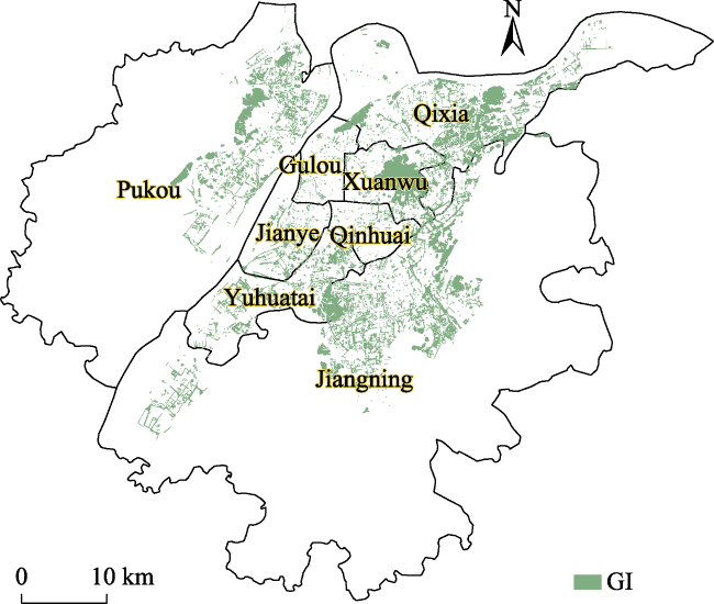
Fig. 2 Green infrastructure (GI) in the main urban area of Nanjing
The second-hand housing sales data were the 89898 second-hand housing price data of 4357 communities in Nanjing in February 2021, which were provided by the Urban Data Party. The data included eight house structure features, including building area, building construction age, building type, house floor, house orientation, house decoration situation, and the number of bedrooms and living rooms. After removing the missing related house structure features and the data with fuzzy information, 18823 observations on 3059 communities remained. Next, datapoints where the walking time to the nearest GI, hospital, supermarket, university, middle school, and primary school exceeded 30 minutes were excluded (the specific operation is in the variable explanation), and finally 2412 valid datapoints were left. The sample points of the communities are shown in Fig. 3.
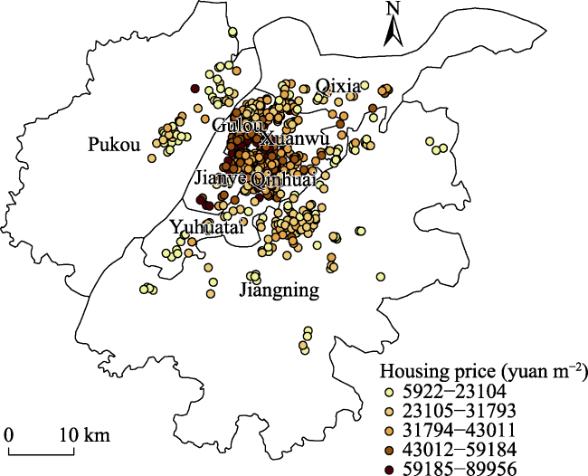
Fig. 3 Sample points of residential area housing prices in the main urban area of Nanjing

3.2 Variables

Following existing studies (Yin et al., 2009), we selected three types of variables: house structure, accessibility, and area. The house structure factors included house construction area, house construction age, building type, house floor, house orientation, house decoration situation, and the number of bedrooms and living rooms. As building type, floor, house orientation, and decoration situation are type variables, we transformed them into quantitative data (Table 1).
Table 1 Variable description
Variable Definition
House
orientation
North is assigned a value of 1; northeast and northwest are assigned a value of 2; east and west are assigned a value of 3; southeast and southwest are assigned a value of 4; and south is assigned a value of 5
House decoration situation Blank room assignment is 1; simple room assignment is 2; and hardcover room assignment is 3
House floor The low floor is assigned a value of 1; the middle floor is as- signed a value of 2; and the high floor is assigned a value of 3
Building type Tower is assigned a value of 1; the combination of slabs and towers is assigned a value of 2; and slabs are assigned a value of 3
The accessibility factors mainly included the distance from the sample point to the nearest GI, hospital, supermarket, university, middle school, and primary school. Using ArcGIS 10.8, these distances between the sample point and the nearest GI, hospital, supermarket, university, middle school, and primary school were first calculated using the OD cost matrix tool in the network analysis module. Then, the distance variable was converted into a time variable with a standard walking speed of 80 m min-1, following existing studies (Shi et al., 2020; Wu and Cheng, 2022). That is, the higher the accessibility, the shorter the time.
Some studies found that urban green space area positively affects housing prices (Yin et al., 2009; Liebelt et al., 2018). Therefore, we selected the area of the nearest GI as the final factor influencing housing prices.

4 Research methods and hypotheses development

4.1 Research methods

4.1.1 Hedonic price model

Since Griliches (1971) and Rosen (1974) created the hedonic price model, it has been widely used in studies to explore the factors influencing housing prices (Xiao et al., 2019; Sohn et al., 2020). Its specific formula is shown below (Yin et al., 2009; Dell’Anna et al., 2022):
$P=P\left(C_{1}, C_{2}, C_{3}, \ldots, C_{n}\right)$
where, P is the housing prices; Cn represents the factors influencing housing prices (e.g., house structure, accessibility, and area); and n is the number of such factors.
Table 2 lists the 15 variables selected and their expected signs for the house structure, accessibility, and area factors.
Table 2 Variable description and expected sign
Groups Variable Definition Expected sign
House structure factor BR Number of bedrooms +
LR Number of living rooms +
AREA Area (m2) +
AGE Age -
ORI House orientation +
DESIGN House decoration situation +
FLOOR House floor +
TYPE Building type
Accessibility factor TPG Time to the nearest GI (min) -
THOS Time to the nearest hospital (min) -
TSUR Time to the nearest supermarket (min) -
TUNI Time to the nearest university (min) -
TMID Time to the nearest middle school (min) -
TPRI Time to the nearest primary school (min) -
Area factor APG The area of the nearest GI (m2) +
At present, the hedonic price model has three main forms: linear, full logarithmic, and semi-logarithmic models (Huang et al., 2021). We cannot use the full logarithmic model as we have many dummy variables. Therefore, we selected the linear (Eq. 2) and semi-logarithmic models (Eq. 3). The linear model is as follows (Tan and Guan, 2021):
P = a 0 + a i C i + ε
The semi-logarithmic model is as follows (Touseef et al., 2021):
ln P = a 0 + a i C i + ε
where, a0 is the constant that affects the price; ai is the characteristic price of the corresponding characteristic variable; and ε is the error term.

4.1.2 Quantile regression model

The quantile regression model was first proposed by Koenker and Bassett (1978), and it is an extension of the traditional ordinary least squares (OLS) regression model (Moreno-Izquierdo et al., 2020). The quantile regression model has the advantage that the regression coefficients are not susceptible to extreme values and the regression results are more robust (Zhang and Yi, 2017). The specific equation used here is shown below (Kang and Liu, 2014):
τ = P y y τ = F y τ
y τ = β 0 + β τ x τ + ε τ
where, τ is the probability; F(y) is the y cumulative probability distribution function; yτ is the τ quantile of y; βτ is the corresponding regression coefficient; xτ is the τ quantile of x; and ετ is the τ quantile of the error term.
Usually, in the quantile regression model, the quantiles τ=0.10, 0.25, 0.50, 0.75, and 0.90 are used to construct the model (Zhang, 2020; Hu and Zhang, 2021). We also used these five quantiles to construct the quantile regression model.

4.2 Hypotheses development

4.2.1 The impact of GI accessibility on housing prices

Marx (2004) noted that land rent refers to the part of the surplus value paid by land users to landowners that is greater than the average profit, i.e., the surplus value of the total land income minus the total cost, including absolute and differential land rents (Wen, 2018). The differential rent can be divided into differential rent I and II (Ma and Yang, 2020). The former is affected by the fertility and quality of the land, while the latter is mainly affected by the labor productivity level of continuous investment in the same land (Deng, 2018). The impact of GI accessibility on housing prices is mainly based on the formation of differential rent II. Specifically, the government invests in GI construction, which drives the development of related industries to a certain extent, so that land prices can be raised, indirectly increasing housing prices (Chen, 2021). Therefore, we can propose our first hypothesis as follows: High accessibility of GI increases the housing prices of surrounding houses.

4.2.2 The different impacts of GI accessibility on the prices of different surrounding houses

People gradually start valuing the quality of the built environment as their income level increases (Su and Yang, 2021). The “Science of Human Settlements” that emerged after 1993 focused on this point (Qi et al., 2006). It emphasizes that there is a relationship between people and the environment: people transform the environment, and the environment also affects human life and activities (Qi et al., 2006). While rapid urbanization has provided convenience for residents to a certain extent, it has also caused problems such as environmental deterioration. Today, the main contradiction in China is the contradiction between the people’s growing need for a better life, but the unbalanced and insufficient development. As economic income and living standards improve, people start demanding higher quality built environments, and are even willing to pay to experience a better environment. Further, as an important resource for improving urban ecological environment, GI can be used to improve the environmental quality in human settlements; however, different groups’ willingness to pay for this may differ. Therefore, we can propose our second hypothesis as follows: The impacts of GI accessibility on the prices of surrounding houses with different prices are different.

5 Results and discussion

5.1 The impact of GI accessibility on surrounding housing prices

As multicollinearity between variables may yield inaccurate regression results, we examined the variance inflation factors (VIF) of all variables before performing the formal regression (Table 3). The corresponding variance expansion coefficient VIF values of all variables were less than 5, which meant that there was no serious multicollinear relationship between the independent variables, and the regression could be performed directly.
Table 3 Variance inflation factors (VIF) of variables
Independent variable VIF Independent variable VIF
BR 3.72 TPG 1.15
LR 1.97 THOS 1.41
AREA 4.17 TSUR 1.31
AGE 1.60 TUNI 1.32
ORI 1.31 TMID 1.26
DESIGN 1.04 TPRI 1.43
FLOOR 1.03 APG 1.37
TYPE 1.23
Next, we used Stata 16 to regress the 2412 housing prices data using the hedonic price model. The regression results in Table 4 shows that the semi-logarithmic model clearly had a better fitting effect; the model using the logarithm of the total price as the dependent variable had the best goodness of fit. The correlation coefficients of the linear and semi-logarithmic models with the total housing prices as the dependent variable were both higher than 0.50, indicating that the accuracy of the two models was higher. Notably, regardless of these two models, the house structure factors of house age, decoration situation, and house floor were significant at the 5% level. Meanwhile, other house structure factors, such as the number of bedrooms, living rooms, area, and house orientation, had different coefficients and significance levels in different models. However, building type was not significant in either model. Among the accessibility factors, the time to the nearest primary school was significant at the 1% level in both models. In the semi-logarithmic model, the time to the nearest GI and universities were significant at the 1% level. This indicates that the GI accessibility significantly affected housing prices. The area of GI also significantly affected housing prices, especially in the semi-logarithmic model where this effect was significant at the 1% level; for every 1% increase in the GI area, housing prices increased by approximately 0.3%.
Table 4 Regression results of the hedonic price model
Independent variable Linear model Semi-logarithmic model
Unit price (UP) Total price (TP) ln (UP) ln (TP)
BR -0.0416 -10.7300** -0.0006 0.0387***
(0.0499) (5.3890) (0.0141) (0.0146)
LR 0.0141 -4.3480 0.0080 0.0595***
(0.0607) (6.5570) (0.0171) (0.0178)
AREA 0.0022* 3.8970*** -0.0001 0.0082***
(0.0013) (0.1370) (0.0004) (0.0004)
AGE 0.0180*** 0.8630** 0.0063*** 0.0032***
(0.0036) (0.3860) (0.0010) (0.0011)
ORI 0.0258 2.4710 0.0057 0.0509***
(0.0300) (3.2430) (0.0085) (0.0088)
DESIGN 0.2800*** 39.7900*** 0.0997*** 0.1090***
(0.0418) (4.5180) (0.0118) (0.0123)
FLOOR -0.1350*** -7.6040** -0.0397*** -0.0318***
(0.0319) (3.4480) (0.0090) (0.0094)
TYPE 0.0044 1.2770 0.0016 0.0018
(0.0417) (4.5060) (0.0118) (0.0122)
TPG 0.0066 0.2390 0.0040*** 0.0058***
(0.0047) (0.5030) (0.0013) (0.0014)
THOS -0.0067 -2.2900 -0.0014 -0.0036
(0.0132) (1.4280) (0.0037) (0.0039)
TSUR 0.0057 1.3910 -0.0012 0.0009
(0.0084) (0.9050) (0.0024) (0.0025)
TUNI -0.0089** -0.0606 -0.0025** -0.0018*
(0.0037) (0.3980) (0.0010) (0.0011)
TMID 0.0002 -0.1910 0.0005 -0.0001
(0.0042) (0.4580) (0.0012) (0.0013)
TPRI -0.0473*** -4.4580*** -0.0121*** -0.0135***
(0.0050) (0.5390) (0.0014) (0.0015)
APG 0.0058** 0.4310 0.0030*** 0.0030***
(0.0025) (0.2690) (0.0007) (0.0007)
Constant 3.1130*** -65.7900*** 1.0070*** 4.2820***
(0.2080) (22.4400) (0.0585) (0.0610)
Observations 2412 2412 2412 2412
R2 0.1030 0.5550 0.1230 0.5670

Note: The unit price of a house means the price of per square meter of a house, and the unit is ten-thousand-yuan m-2, and the unit of the total housing prices is ten thousand yuan. *** P < 0.01, ** P < 0.05, and * P < 0.1.

5.2 The impact of GI accessibility on housing prices at different price levels

As the model with total housing prices as the dependent variable had a better fit in Table 4, total housing prices was also selected as the dependent variable in the quantile regression model. Table 5 shows that GI accessibility had a significant impact on different housing price levels, especially in the 25%-90% range. Moreover, the impact increased as the housing prices increased. In the top 90% of the housing prices, for every 1 minute increase in the time to the nearest GI, the average price of the house decreased by approximately 9760 yuan; in the top 75% of the housing prices, for every 1 minute increase in the time to the nearest GI, the average price dropped by about 14370 yuan; in the top 50% of the housing prices, for every 1 minute increase in the time to the nearest GI, the average price of the house dropped by about 22930 yuan; in the top 25% of the housing prices, for every 1 minute increase in the time to the nearest GI, the average price of the house dropped by about 35990 yuan. However, in the top 10% of housing prices, GI accessibility had no significant impact on housing prices; moreover, the coefficient decreased. This may be because the environment of the community itself was very good. Therefore, people’s demand for GI around such communities may not be high. In summary, housing prices were negatively related to the GI accessibility; as the income level increases, people would be willing to pay more to live near GI.
Table 5 Linear-quantile model regression results
Independent variable Linear model
10% 25% 50% 75% 90%
BR -27.1800 -31.2000*** -30.8900*** -26.0900*** -18.8200***
(17.7300) (11.5400) (7.7560) (6.1910) (5.5750)
LR -27.1100 -44.7400*** -25.7800** -16.7000** -10.5900
(25.8800) (16.3800) (10.0500) (7.5540) (6.8310)
AREA 3.1660*** 3.4160*** 3.9690*** 4.2320*** 4.2000***
(0.4120) (0.2640) (0.1880) (0.1540) (0.1410)
AGE -13.8600*** -6.6200*** -0.9450 0.3290 0.4350
(2.4880) (1.2450) (0.7000) (0.4720) (0.4010)
ORI -21.3300 -8.4050 8.0150 4.9670 3.8200
(23.8500) (15.5300) (9.1860) (5.2430) (4.0980)
DESIGN 46.3900** 53.5900*** 34.4800*** 31.7500*** 31.4800***
(21.0600) (11.9700) (7.2510) (5.3700) (4.7420)
FLOOR 10.1600 17.8100** 5.3520 -5.1800 -8.0180**
(14.3000) (8.3270) (5.3750) (4.0780) (3.5840)
TYPE -0.1980 6.9070 -4.0770 -0.8700 -4.8370
(19.1400) (11.3000) (7.4250) (5.5120) (4.8440)
TPG -0.0123 -3.5990*** -2.2930*** -1.4370** -0.9760*
(2.6970) (1.2760) (0.8250) (0.6080) (0.5280)
THOS -17.7900*** -6.3130** -3.9650* -2.6280 -2.9800**
(5.7230) (3.1470) (2.1540) (1.7140) (1.5110)
TSUR -15.7000*** -5.0030* 5.0870*** 3.3290*** 2.2040**
(5.1700) (2.6710) (1.5890) (1.1240) (0.9390)
TUNI 2.3130 -1.0190 0.6710 0.7760 0.2800
(1.8580) (0.9740) (0.6430) (0.4800) (0.4180)
TMID 2.7630 0.2110 -2.1610*** -1.0030* -0.6350
(2.1910) (1.2130) (0.7910) (0.5620) (0.4910)
TPRI -7.5750*** -5.4200*** -5.6500*** -5.4340*** -4.8960***
(2.3620) (1.3480) (0.8650) (0.6330) (0.5660)
APG -3.0530 -2.8740*** -0.8540** 0.0584 0.3210
(1.9440) (0.6450) (0.3510) (0.2920) (0.2700)
Constant 736.3000*** 433.0000*** 125.8000** 20.3000 -1.0190
(171.0000) (96.3700) (52.4400) (31.0600) (25.2600)
Observations 241 603 1206 1809 2171
R2 0.4700 0.3930 0.4470 0.5220 0.5560

Note: *** P < 0.01, ** P < 0.05, and * P < 0.1.

The semi-log-quantile model results could better reflect the impact of GI accessibility on houses at different price levels. It could be seen from Table 6 that GI accessibility significantly affects housing prices, especially in the range of 25%-75% of housing prices. In the top 75% of housing prices, for every 1% increase in the time to the nearest GI, the total housing prices dropped by an average of approximately 0.31%; in the top 50% of housing prices, for every 1% increase in the time to the nearest GI, the total price dropped by approximately 0.54% on average; in the top 25% of housing prices, for every 1% increase in the time to the nearest GI, the total housing prices dropped by approximately 0.64% on average. However, no significant impacts were observed in the top 10% and 90%. For the top 10% housing prices, the environment of the community itself may be very good; thus, they may not need more GI. Meanwhile, among the 90%, people with lower housing prices may not be willing to pay for GI.
Table 6 Regression results of semi-log-quantile model
Independent variable Semi-logarithmic model
10% 25% 50% 75% 90%
BR -0.0261 -0.0404*** -0.0421*** -0.0290** 0.0014
(0.0181) (0.0155) (0.0137) (0.0132) (0.0133)
LR -0.0155 -0.0417* -0.0221 0.0043 0.0311*
(0.0264) (0.0221) (0.0177) (0.0162) (0.0163)
AREA 0.0031*** 0.0044*** 0.0065*** 0.0082*** 0.0086***
(0.0004) (0.0004) (0.0003) (0.0003) (0.0003)
AGE -0.0158*** -0.0085*** -0.0005 0.0011 0.0006
(0.0025) (0.0017) (0.0012) (0.0010) (0.0010)
ORI -0.0314 -0.0129 0.0188 0.0255** 0.0258***
(0.0244) (0.0209) (0.0162) (0.0112) (0.0098)
DESIGN 0.0424* 0.0715*** 0.0604*** 0.0701*** 0.0761***
(0.0215) (0.0161) (0.0128) (0.0115) (0.0113)
FLOOR 0.0131 0.0242** 0.0064 -0.0227*** -0.0349***
(0.0146) (0.0112) (0.0095) (0.0087) (0.0086)
TYPE 0.0060 0.0179 -0.0077 0.0010 -0.0164
(0.0196) (0.0152) (0.0131) (0.0118) (0.0116)
TPG 0.0001 -0.0064*** -0.0054*** -0.0031** -0.0006
(0.0028) (0.0017) (0.0015) (0.0013) (0.0013)
THOS -0.0168*** -0.0060 -0.0046 -0.0030 -0.0052
(0.0059) (0.0042) (0.0038) (0.0037) (0.0036)
TSUR -0.0167*** -0.0053 0.0122*** 0.0066*** 0.0036
(0.0053) (0.0036) (0.0028) (0.0024) (0.0022)
TUNI 0.0016 -0.0018 0.0019* 0.0022** 0.0001
(0.0019) (0.0013) (0.0011) (0.0010) (0.0010)
TMID 0.0035 0.0012 -0.0030** -0.0001 0.0003
(0.0022) (0.0016) (0.0014) (0.0012) (0.0012)
TPRI -0.0084*** -0.0083*** -0.0114*** -0.0140*** -0.0131***
(0.0024) (0.0018) (0.0015) (0.0014) (0.0014)
APG -0.0030 -0.0040*** -0.0013** 0.0013** 0.0023***
(0.0020) (0.0009) (0.0006) (0.0006) (0.0006)
Constant 6.6330*** 6.1060*** 5.3970*** 4.9260*** 4.7630***
(0.1750) (0.1300) (0.0926) (0.0664) (0.0604)
Observations 241 603 1206 1809 2171
R2 0.4790 0.3810 0.4420 0.5310 0.5680

Note: *** P < 0.01, ** P < 0.05, and * P < 0.1.

6 Conclusions

We examined the impact of GI accessibility on housing prices, and the heterogeneity of this impact across different housing prices. Data on housing characteristics and prices in Nanjing were analyzed using the hedonic price and quantile regression models. The findings are summarized below:
(1) GI accessibility had a significant impact on housing prices, and the semi-logarithmic model results were better than the linear model; in addition, every 1% increase in GI area increased housing prices by approximately 0.3%. The results of the hedonic price model (Table 4) indicated that the house structure factor was the main factor affecting the housing price. Other external factors also had a significant impact on the housing price, such as the distance to primary school.
(2) The impacts of GI accessibility on different housing price levels were different; that is, the sensitivity to GI accessibility was different at different housing price levels. This was especially true in the 25%-75% housing price range, where housing prices were negatively correlated with the GI accessibility. This showed that residents with a certain economic strength wanted to live near GI.
Finally, this study has some limitations: First, we did not examine the impact of GI construction on housing prices. Second, given limits to data collection, we did not consider the impact of location factors in regression analysis. This will to some extent affect the analysis results, but will not fundamentally affect the effectiveness of the results.
[1]
Berland A, Shiflett S A, Shuster W D, et al. 2017. The role of trees in urban stormwater management. Landscape and Urban Planning, 162: 167-177.

DOI PMID

[2]
Chen T. 2021. Research on the impact of urban park green space in Urumqi City on the price of surrounding residential buildings. Diss., Urumqi, China: Xinjiang University of Finance & Economics. (in Chinese)

[3]
Conway T M, Khan A, Esak N. 2020. An analysis of green infrastructure in municipal policy: Divergent meaning and terminology in the Greater Toronto Area. Land Use Policy, 99: 104864. DOI: 10.1016/j.landusepol.2020.104864.

[4]
Dell’Anna F, Bravi M, Bottero M. 2022. Urban green infrastructures: How much did they affect property prices in Singapore? Urban Forestry and Urban Greening, 68: 127475. DOI: 10.1016/j.ufug.2022.127475.

[5]
Deng Y D. 2018. Research on the formation of urban house price in China based on Marx’s Land Rent Theory. China Economic Studies, 311(6): 3-12. (in Chinese)

[6]
Gao Z B, Wang X R, Sui X Y, et al. 2022. Multi-scenario prediction of habitat quality in Nanjing based on FLUS and InVEST models. Journal of Agricultural Resources and Environment, 39(5): 1001-1013. (in Chinese)

[7]
Griliches Z. 1971. Price indexes and quality change. Cambridge, USA: Harvard University Press.

[8]
Hoover F A, Price J I, Hopton M E. 2020. Examining the effects of green infrastructure on residential sales prices in Omaha, Nebraska. Urban Forestry and Urban Greening, 54: 126778. DOI: 10.1016/j.ufug.2020.126778.

[9]
Hu W, Zhang J H. 2021. The power of cities: Hierarchical migration and wage premium of migrant workers. Journal of Finance and Economics, 47(2): 4-18. (in Chinese)

[10]
Huang C C, Wang X W, Li L N. 2021. The spatio-temporal effects of urban rail transit on housing price: A case study of Fuzhou Metro Line 1. Geographical Research, 40(10): 2808-2822. (in Chinese)

DOI

[11]
Kang H H, Liu S B. 2014. The impact of the 2008 financial crisis on housing prices in China and Taiwan: A quantile regression analysis. Economic Modelling, 42: 356-362.

DOI

[12]
Koenker R, Bassett Jr G. 1978. Regression quantiles. Econometrica, 46(1): 33-50.

DOI

[13]
Li K M, Li C L, Cao J J, et al. 2021. Spatiotemporal evolution characteristics of urban green infrastructure in central Liaoning urban agglomeration during the past 20 years based on landscape ecology and morphology. Acta Ecologica Sinica, 41(21): 8408-8420. (in Chinese)

[14]
Liebelt V, Bartke S, Schwarz N. 2018. Hedonic pricing analysis of the influence of urban green spaces onto residential prices: The case of Leipzig, Germany. European Planning Studies, 26(1): 133-157.

DOI

[15]
Liu Y X, Chen T. 2020. Impact of urban park green space on the price of peripheral housing in Urumqi. Journal of Arid Land Resources and Environment, 34(11): 36-43. (in Chinese)

[16]
Ma Y, Yang H. 2020. Educational differential land rent of school distinct housing and the effect of unequal educational opportunities. Journal of Finance and Economics, 46(5): 37-51. (in Chinese)

[17]
Marx. 2004. Capital: Volume 3. Beijing, China: People’s Publishing House. (in Chinese)

[18]
Moreno-Izquierdo L, Rubia-Serrano A, Perles-Ribes J F, et al. 2020. Determining factors in the choice of prices of tourist rental accommodation: New evidence using the quantile regression approach. Tourism Management Perspectives, 33: 100632. DOI: 10.1016/j.tmp.2019.100632.

[19]
Nazir N N M, Othman N, Nawawi A H. 2015. Role of green infrastructure in determining house value in Labuan using hedonic pricing model. Procedia-Social and Behavioral Sciences, 170: 484-493.

[20]
Qi X H, Mao J X, Cheng Y, et al. 2006. Development of theoretical study on human settlement in China since reform and opening up. Planners, (8): 14-16. (in Chinese)

[21]
Rosen S. 1974. Hedonic prices and implicit markets: Product differentiation in pure competition. Journal of Political Economy, 82(1): 34-55.

DOI

[22]
Shi F, Zhu L, Yuan R. 2020. Progress of public transport accessibility analysis methods. Human Geography, 37(6): 20-29, 46. (in Chinese)

[23]
Sohn W, Kim H W, Kim J H, et al. 2020. The capitalized amenity of green infrastructure in single-family housing values: An application of the spatial hedonic pricing method. Urban Forestry and Urban Greening, 49: 126643. DOI: 10.1016/j.ufug.2020.126643.

[24]
Su J H, Yang Y. 2021. Research on micro-renewal strategies of old communities under the scientific theory of human settlement environment—A case of Zhuanxin Farmers’ Market Area in Kunming. Urbanism and Architecture, 18(1): 34-38. (in Chinese)

[25]
Suppakittpaisarn P, Jiang B, Slavenasc M, et al. 2019. Does density of green infrastructure predict preference? Urban Forestry and Urban Greening, 40: 236-244.

DOI

[26]
Tan M J, Guan C H. 2021. Are people happier in locations of high property value? Spatial temporal analytics of activity frequency, public sentiment and housing price using twitter data. Applied Geography, 132: 102474. DOI: 10.1016/j.apgeog.2021.102474.

[27]
Touseef H, Jaffar A, Zou W, et al. 2021. Impact of urban village disamenity on neighboring residential properties: Empirical evidence from Nanjing through Hedonic Pricing Model appraisal. Journal of Urban Planning and Development, 147(1): 0000645. DOI: 10.1061/(asce)up.1943-5444.0000645.

[28]
Wang X, Qin S S. 2021. On Xi Jinping’s ecological civilization thought from the perspective of environmental governance modernization. Journal of Chongqing University (Social Science Edition), 27(1): 227-237. (in Chinese)

[29]
Wen B Y. 2018. Study on the impact of urban ecological landscape on housing price—In case of Wuhan. Diss., Wuhan, China: Huazhong Agricultural University. (in Chinese)

[30]
Wu Z, Cheng X L. 2022. Study on the distribution and accessibility of public service facilities in Fengyang County from the perspective of community life circle. Architecture & Culture, 225(12): 69-71. (in Chinese)

[31]
Xiao Y, Hui E C M, Wen H Z. 2019. Effects of floor level and landscape proximity on housing price: A hedonic analysis in Hangzhou, China. Habitat International, 87: 11-26.

DOI

[32]
Yin H W, Xu J G, Kong F H. 2009. Impact of the amenity value of urban green space on the price of house in Shanghai. Acta Ecologica Sinica, 29(8): 4492-4500. (in Chinese)

[33]
Zhang L, Yi Y M. 2017. Quantile house price indices in Beijing. Regional Science and Urban Economics, 63: 85-96.

DOI

[34]
Zhang T. 2020. Forecast of daily rent price of shared accommodation based on hedonic price method—A case study of Beijing Airbnb shared accommodation. Diss., Beijing, China: Beijing Jiaotong University. (in Chinese)

Outlines

/