
Journal of Resources and Ecology >
Effect of China’s Taiwan Agricultural Investment in China’s Mainland: Based on the Model of VAR and VEC
|
LI Hangfei, E-mail: lihangfei1980@126.com |
Received date: 2022-10-13
Accepted date: 2023-04-30
Online published: 2024-03-14
Supported by
The National Natural Science Foundation of China(41771136)
The Philosophy and Social Science Planning Project of Guangdong(GD22CYJ26)
The Science and Technology Planning Project of Shaoguan(200811154532282)
Based on the data from the 1991-2016 agricultural investment of China’s Taiwan in China’s Mainland and the agricultural GDP of the latter, through models of vector autoregressive (VAR) and vector error correction (VEC), the influences of China’s Taiwan agricultural investment on the development of agriculture in the eastern, central, and western regions of China are discussed. The results show a long-term equilibrium relationship between China’s Taiwan agricultural investment and agricultural development in China’s eastern, central, and western regions. In the long term, China’s Taiwan investment in agriculture in the eastern, central, and western regions of China have certain positive promoting effect on their agricultural development. However, there is an obvious regional diversity in investment effect: Impulse response and variance decomposition show that the positive effect from China’s Taiwan agricultural investment in China’s western region agricultural development is most significant, and it is significantly higher than that in the eastern region; its contribution to the central region’s agricultural development is little. VEC model analysis shows that in the short term, China’s Taiwan investment in agriculture has a significant positive effect on the agricultural development of China’s eastern region, but not on the agricultural development of the central and western regions.
Key words: China’s Taiwan; agricultural investment; VAR model; China’s Mainland; VEC model
LI Hangfei , YANG Lin . Effect of China’s Taiwan Agricultural Investment in China’s Mainland: Based on the Model of VAR and VEC[J]. Journal of Resources and Ecology, 2024 , 15(2) : 293 -303 . DOI: 10.5814/j.issn.1674-764x.2024.02.005
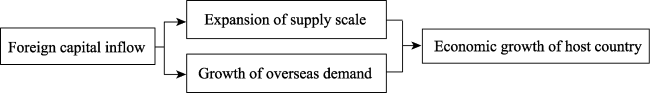
Fig. 1 Traditional economic growth theory |
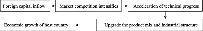
Fig. 2 New economic growth theory |
Table 1 Agricultural location quotient and agricultural fixed asset investment in the eastern provinces of China |
| Province | Liaoning | Beijing | Tianjin | Hebei | Shandong | Shanghai |
|---|---|---|---|---|---|---|
| Agricultural location quotient | 1.135805 | 0.058794 | 0.143173 | 1.266402 | 0.842571 | 0.045173 |
| Proportion of fixed assets investment in agriculture (%) | 3.664557 | 1.317541 | 2.542282 | 5.591442 | 2.957974 | 0.060525 |
| Province | Jiangsu | Zhejiang | Fujian | Guangdong | Hainan | China |
| Agricultural location quotient | 0.612612 | 0.483604 | 0.953792 | 0.531295 | 2.720647 | 1 |
| Proportion of fixed assets investment in agriculture (%) | 0.969081 | 1.430189 | 3.839435 | 1.625406 | 1.461739 | 4.134692 |
Note: 1. Agricultural location quotient = (Provincial agricultural GDP/ Provincial GDP) / (National agricultural GDP/ National GDP). If the value is greater than one, agriculture has an industrial comparative advantage; if the value is less than one, there is no industrial comparative advantage. 2. Proportion of fixed investment in agriculture = (Fixed asset investment in agriculture, forestry, animal husbandry, and fishery)/fixed asset investment in society. |
Fig. 3 Regions distribution of China’s Taiwan agricultural investment in China’s Mainland |
Table 2 Unit root tests of variables |
| Inspection form (c, t, p) | ADF | Critical value (1%) | Critical value (5%) | Critical value (10%) | Inspection conclusion | |
|---|---|---|---|---|---|---|
| D2LNDB | (c, t, 1) | ‒5.750585 | ‒4.440739 | ‒3.632896 | ‒3.254671 | Smooth |
| D2LNDBTW | (c, 0, 1) | ‒6.198601 | ‒3.857386 | ‒3.040391 | ‒2.660551 | Smooth |
| D2LNZB | (c, 0, 1) | ‒5.422502 | ‒3.769597 | ‒3.004861 | ‒2.642242 | Smooth |
| D2LNZBTW | (c, 0, 1) | ‒14.67004 | ‒3.769597 | ‒3.004861 | ‒2.642242 | Smooth |
| DLNXB | (c, 0, 0) | ‒4.994655 | ‒3.857386 | ‒3.040391 | ‒2.660551 | Smooth |
| DLNXBTW | (c, 0, 0) | ‒4.048867 | ‒3.857386 | ‒3.040391 | ‒2.660551 | Smooth |
Note: 1. D2LNDB, D2LNDBTW, D2LNZB and D2LNZBTW are the second-order differences in LNDB, LNDBTW, LNZB and LNZBTW, respectively; DLNXB and DLNXBTW are the first-order differences in LNXB and LNXBTW, respectively; 2. In the test form, c is the intercept term, t is the time trend term and p is the lag order. |
LNDB = 1.259708 × LNDBTW + 0.701125 + ε
LNZB = 0.839251 × LNZBTW + 6.868914 + ε
LNXB = 1.568386 × LNXBTW + 1.427074 + ε
Table 3 Granger causality tests |
| Null hypothesis | Lag length | F statistic | P values | Inspection results |
|---|---|---|---|---|
| LNDBTW does not granger cause LNDB | 4 | 3.01650 | 0.0579 | Reject null hypothesis |
| LNZBTW does not granger cause LNZB | 2 | 0.95515 | 0.4025 | Accept null hypothesis |
| LNXBTW does not granger cause LNXB | 1 | 6.12932 | 0.0249 | Reject null hypothesis |
Note: Hysteresis length is the optimal hysteresis length in the corresponding VAR model. |
Table 4 VAR lag order selection criteria |
| Lag | LOGL | LR | FPE | AIC | SC | HQ |
|---|---|---|---|---|---|---|
| 0 | ‒1.010715 | NA | 0.004508 | 0.273701 | 0.372887 | 0.297067 |
| 1 | 74.44040 | 130.3247 | 6.83e‒06 | ‒6.221855 | ‒5.924298 | ‒6.151759 |
| 2 | 80.27560 | 9.018038 | 5.85e‒06 | ‒6.388691 | ‒5.892763 | ‒6.271865 |
| 3 | 84.92929 | 6.345931 | 5.68e‒06 | ‒6.448117 | ‒5.753817 | ‒6.284561 |
| 4 | 100.5206 | 18.42614* | 2.10e‒06* | ‒7.501876* | ‒6.609204* | ‒7.291589* |
Note: * represents the lag order of the model selected according to the corresponding criteria; NA represents no data. |
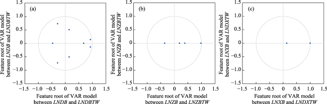
Fig. 4 The stability test of VAR modelNote: The scale indicates the size of the feature root in the VAR model. |
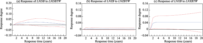
Fig. 5 Response of LNDB, LNZB, LNXB to LNDBTW, LNZBTW, LNXBTW, respectivelyNote: The solid line is the impulse response function curve, and the dashed line is the plus or minus double standard deviation band. |
Fig. 6 Variance decomposition of LNDB, LNZB, LNXB |
D(LNDBt)=‒0.101058×ECMt‒1+0.464069×D(LNDBt‒1)‒
0.119821×D(LNDBt‒2)+0.279823×
D(LNDBt‒3)+0.122802×D(LNDBTWt‒1)+
0.030759×D(LNDBTWt‒2)+0.22718×
D(LNDBTWt‒3) ‒0.003010
ECMt=LNDBt‒1.259708×LNDBTWt‒0.701125
R2= 0.602820, AIC=‒7.326158, SC=‒6.433487
D(LNZBt) =‒0.048417×ECMt‒1 +0.325053×D(LNZBt‒1)+
0.031958×D(LNZBTWt‒1)+0.032099
ECMt= LNZBt‒0.839251×LNZBTWt‒6.868914
R2= 0.158449, AIC=‒5.280502, SC=‒4.789646
D(LNXBt)=‒0.397962×ECMt‒1‒0.158504×D(LNXBt‒1)+
0.119645×D(LNXBTWt‒1)+0.078769
ECMt= LNXBt‒1.568386×LNXBTWt‒1.427074
R2= 0.296788, AIC=‒5.030768, SC=‒4.536117
| [1] |
|
| [2] |
|
| [3] |
|
| [4] |
|
| [5] |
|
| [6] |
|
| [7] |
|
| [8] |
|
| [9] |
|
| [10] |
|
| [11] |
|
| [12] |
|
| [13] |
|
| [14] |
|
| [15] |
|
| [16] |
|
| [17] |
|
| [18] |
|
| [19] |
|
| [20] |
|
| [21] |
|
| [22] |
|
| [23] |
|
| [24] |
|
| [25] |
|
| [26] |
|
| [27] |
|
| [28] |
|
| [29] |
|
| [30] |
|
| [31] |
|
| [32] |
|
| [33] |
|
| [34] |
|
| [35] |
|
| [36] |
|
| [37] |
|
| [38] |
|
| [39] |
|
| [40] |
|
/
| 〈 |
|
〉 |

