Agroecology and Agricultural Development

Agricultural Total Factor Productivity based on Farmers’ Perspective: An Example of CCR, BCC, SBM and Technology Optimization Malmquist-Luenberger Index

  • CHENG Yongsheng , 1, 2, 3 ,
  • ZHANG Deyuan 2 ,
  • WANG Xia 3
Expand
  • 1. School of Business, Fuyang Normal University, Fuyang, Anhui 236037, China
  • 2. Academy of Strategies for Innovation and Development, Anhui University, Hefei 230601, China
  • 3. School of Economics, Fuyang Normal University, Fuyang, Anhui 236037, China

CHENG Yongsheng, E-mail:

Received date: 2022-09-26

  Accepted date: 2023-04-30

  Online published: 2024-03-14

Supported by

The Philosophy and Social Science Foundation of Anhui Province(AHSKQ2022D039)

Abstract

Based on a large national sample of the China Family Panel Studies (CFPS) database, the study will to provide some thoughts and suggestions for the transformation and upgrading of China’s agriculture, the enhancement of total factor productivity by exploring the agricultural production efficiency from the micro-farmers’ perspective. By constructing the models of Charnes, Cooper & Rhodes (CCR), Banker, Charnes & Cooper (BCC), Slacks-Based Model (SBM) and technology optimization Malmquist-Luenberger index, it finally obtained the comprehensive technical efficiency value, pure technical efficiency value, farm household efficiency value and green total factor productivity level value at the micro-farm household level based on the comparative analysis. It was found that: the comparison of the measures based on different models found that although there are differences in the calculated efficiency values, the pure technical efficiency values calculated by BCC are the main factors affecting the micro agricultural production efficiency values at the farmer level, the SBM model should optimize the CCR, BCC models, and more suitable for Chinese government policy formulation and optimization; the technology optimization Malmquist-Luenberger index method is the micro agricultural production efficiency measurement method of choice, with the characteristics of diverse model selection, rich application scenarios and convenient processing of negative outputs; environmental factors in the current evaluation of agricultural green total factor productivity, mainly play a negative inhibitory role, reducing the negative externalities of environmental variables output, become one of the key issues facing the current micro farm layer green total factor production enhancement; the combination of subjective and objective measures of environmental non-desired output is an important way to measure environmental factors of agricultural green total factor productivity, it can be used in practical applications based on a combination of research objectives and data availability.

Cite this article

CHENG Yongsheng , ZHANG Deyuan , WANG Xia . Agricultural Total Factor Productivity based on Farmers’ Perspective: An Example of CCR, BCC, SBM and Technology Optimization Malmquist-Luenberger Index[J]. Journal of Resources and Ecology, 2024 , 15(2) : 267 -279 . DOI: 10.5814/j.issn.1674-764x.2024.02.003

1 Introduction

Productivity is an eternal fundamental theme in economic and social development, analyzing the inner laws of economic development from the perspective of micro-subjectivity such as enterprises has become one of the hot topics of research in recent years. After all, productivity is the decisive factor for micro-subjects to enter or exit the market (Song, 2021), and agricultural production is no exception. The efficiency evaluation from the perspective of total factor productivity is to extend the index from single input to multiple input and to include the consideration of the coordination effect among different input factors, which better covers the connotation of efficiency and can analyze the efficiency issue more comprehensively and objectively, it is also more in line with the real economic and social development, whose official version first appeared in the report of the 19th National Congress of the Communist Party of China and the “14th Five-Year Planning” emphasizes the need to build a new pattern with total factor productivity improvement to promote high-quality development of China’s economy (Guo et al., 2022). The 20th National Congress of the Communist Party of China further clarified the focus on improving total factor productivity to promote the economy to achieve effective quality improvement and reasonable quantitative growth, which fits the current profound connotation of high-quality development as the first task of building a modern socialist country in a comprehensive manner. As a quantifiable observation indicator, agricultural total factor productivity not only measures the efficiency of utilization of factor inputs of farmers, but also reveals the comprehensive efficiency of micro agricultural development, which can reflect the current level of agricultural modernization. China is a large agricultural country, the issue of “three rural areas” has always been a fundamental issue in the development of the country, it is a shortcoming in the realization of a fully built socialist modern country, and a bottleneck in the realization of common prosperity. How to accelerate the transformation and upgrading of agriculture and effectively improve total factor productivity is a major task for the current and future development of China. Therefore, on the basis of accurately grasping the core meaning, the scientific measurement of agricultural total factor productivity becomes an inevitable prerequisite for exploring the path of agricultural modernization and building a strong agricultural country.
From the established literature, the traditional methods of measuring and analyzing total factor productivity can be generally distinguished into macro and micro two levels of discussion. Specifically, in terms of macro level, there are parametric analysis methods represented by Solow Complementary Method (SCM), Stochastic Frontier Approach (SFA) and Data Envelopment Analysis (DEA) method, which is the most typical representative of non-parametric methods (Cheng, 2022).
At the micro level, the existing domestic and foreign literature on total factor productivity research mainly focuses on the enterprise level, a large number of more mature research results have been formed on total factor productivity research represented by the manufacturing industry. Among the more common methodological applications, including the application of parametric and semi-parametric methods to develop productivity accounting for industrial enterprises, such as least squares, fixed effects, OP and LP methods, etc. The leading idea is to use intermediate inputs as instrumental variables to address the endogeneity treatment, sample selectivity bias possibility of the econometric model. Further to the agricultural total factor productivity, there is a relative lack of studies, especially those based on micro data (Wang et al., 2020), and the few studies that use micro data to measure the productivity of farm households use the OP method (Wang et al., 2020; Chari et al., 2021), the LP method (Zhu et al., 2018) and especially the DEA method (Wang et al., 2017; Zhang, 2018; Huang and Ma, 2021), the limited studies based on different research perspectives and measurement methods have not reached a consensus on the findings from the literature crawl (Li et al., 2010; Li and Yin, 2017; Huang and Ma, 2021).

2 Model construction

DEA analysis is a non-parametric technical efficiency analysis method implemented from the relativity between the evaluated objects (decision units), based on a linear programming basis and a distance function approach to model evaluation, which first appeared in 1978 and was also named the CCR model because the model was first proposed by Charnes, Cooper and Rhodes in the United States (Charnes et al., 1978). Because of its broad scope of application, its relatively simple methodological principle, and especially its special inherent advantages in analyzing multiple inputs and outputs, which are more in line with the real production process, it has been rapidly expanded to many research fields since its introduction.

2.1 CCR model based on constant returns to scale

DEA generally refers to the object of the efficiency measure as a decision making unit (DMU), assuming that there are n DMUs, denoted as D M U j   j = 1 , 2 , , n, each DMU has m inputs, denoted as x i   i = 1 , 2 , , m, and q outputs, denoted as y r   r = 1 , 2 , , q, then the linear programming form of the output-oriented CCR-based model can be expressed as:
max φ s . t . j = 1 n λ j x i j x i k     j = 1 n λ j y r j φ y r k     j , λ j 0 i = 1 , 2 , , m ; r = 1 , 2 , , q ; j = 1 , 2 , , n  
Specifically, φ is the optimal solution of the model; n  is the number of decision units; k denotes the decision unit currently located; m and q denote the total number of inputs and outputs of each decision unit, respectively; j, i, r denote the ordinal numbers of decision units, inputs and outputs, respectively; λj is the linear combination coefficient between decision units. The above Equation (1) is expressed to show that based on the given input conditions, each output term can be used to measure the inefficiency using the degree of equal proportional increase, so it is also called the output-oriented CCR model. Assuming that based on the current technology level, the decision making unit D M U k takes the premise of no increase in inputs, then φ 1 is the maximum proportion of its output can be increased; if φ is larger, it means that its output can be increased accordingly, and the efficiency is correspondingly lower, generally using 1 / φ to reflect its efficiency value.

2.2 BCC model based on variable returns to scale

The above CCR model assumes constant returns to scale for the production technology, it is predetermined that all decision units DMUs are at the optimal production scale stage. However, it is obvious that in the real production process, many production units are not, and cannot be at the optimal scale of production. For this reason, Banker, Charnes and Cooper proposed the BCC model in 1984, subsequently named after them, which is also known as pure technical efficiency because the technical efficiency derived from this model excludes the effect of production scale. Based on the CCR model, the BCC model is composed with the addition of the constraint j = 1 n λ j = 1 λ 0, and the linear programming form of the output-oriented BCC-based model can be specified by the following equation:
max ϕ s . t . j = 1 n λ j x i j x i k           j = 1 n λ j y r j ϕ y r k           j = 1 n λ j = 1 j , λ j 0 i = 1 , 2 , , m ; r = 1 , 2 , , q ; j = 1 , 2 , , n
In the above Equation (2), ϕ denotes the optimal solution of the model, and the interpretation of other variables is the same as that of Equation (1), which is not repeated here.

2.3 SBM model based on slack variables

The commonality of the above-mentioned CCR model and BCC model lies in the realization of the improvement of the ineffective DMU, that is the equal proportional reduction (increase) of all inputs (outputs), and they all belong to the radial DEA model. However, in terms of the reality of production practice, the gap between the current state of the ineffective DMU and the strong effective target value may include not only the part with equal proportional improvement, but also the part with slack improvement. Based on such considerations, the Slack-Based Measure (SBM) model was then proposed by Tone in 2001, with the significant advantage of achieving a better solution to the problem that the radial model does not include slack variables in the measurement of inefficiency. The matrix form of the planning equation is:
min ρ s . t . X λ + s = x k Y λ s + = y k λ , s , s + 0
In the above Equation (3), ρ = 1 1 m i = 1 m s i / x i k / 1 + 1 q r = 1 q s r + / y r k, ρ  expresses the efficiency value of the DMU under evaluation, and it can measure the inefficiency in both input and output dimensions, so it is also called the non-oriented model. If ρ = 1, it means that the evaluated DMU is strongly efficient. where X and Y are the elements in the corresponding input and output matrices, s and s+ are the input and output slack variables, and λ is the weight vector; the other variables are explained as in Equation (1).

2.4 Malmquist-Luenberger index measure for technology optimization

Of course, the CCR model, the BCC model and the SBM model are not perfect, but their common shortcoming is that they do not take into account the negative outputs (non-desired outputs) in the production process. Generally speaking, there is a concomitant relationship between positive and negative outputs, and the “bad” products are produced at the same time as the “good” products are produced. In order to solve this problem, scholars (Chung et al., 1997) further improved the Malmquist-Luenberger index (M-L index) based on the Directional Distance Function (DDF), which has the advantage of increasing positive output and decreasing negative output at the same time,but it has method suffers from inconsistency and non-feasibility problems, which may lead to biased measurements. In view of this, Aparicio et al. (2017) introduced optimization techniques based on the above M-L index to overcome the inconsistency and non-feasibility problems that arise in the measurement process (Cheng et al., 2022).
Assuming that the DMU input is x R + N, the positive output is y R + M, the negative output is b R + I, the set of production technologies is P t x t:

P t x t = y , b R + M × R + I k = 1 K z k y k m t y m , m = 1 , 2 , , M k = 1 K z k b k i t b i , i = 1 , 2 , , I k = 1 K z k x k m t x n t , n = 1 , 2 , , N b i b ¯ i t x t , i = 1 , 2 , , I z k 0 , k = 1 , 2 , , K

In the above Equation (4), the variables M, I and N denote the number of desired outputs (y), non-desired outputs (b), and inputs (x), respectively; and K denotes the number of parameters to be determined (zk); t denotes the period, b ¯ i t x t denotes the upper bound value of negative output. The directional distance function D o x , y , b ; g = s u p β : y , b + β g P x, g is introduced as the directional vector, and in general, let g = y , b, denote an increase in positive output and a decrease in negative output. The M-L index of technology optimization is defined as:
M L s = 1 + D o s x t , y t , b t ; y t , b t 1 + D o s x t + 1 , y t + 1 , b t + 1 ; y t + 1 , b t + 1

s = t , t + 1

In the above Equation (5), it can be further decomposed into the product of the green technical efficiency change (MLTEC), and the green technical progress change (MLTC). The green technical efficiency change represents the distance between the DMU and the production frontier, the catch-up effect reflecting the degree of improvement in the resource allocation, management mode and organization of the DMU; while the green technical progress change represents the moving state of the production frontier, the frontier transformation effect expressing the technological innovation process promoted by the DMU through the external introduction of technology and internal innovation of technology. In order to avoid the arbitrariness in the choice of reference technology frontier surface, the M-L indexes of the two periods are taken as geometric averages.
max β = D o s x o h , y o h , b o h ; y o h , b o h s . t . k = 1 K z k y k m s y o m h + β y o m h , m = 1 , 2 , , M k = 1 K z k b k i s b o i h β b o i h , i = 1 , 2 , , I k = 1 K z k x k n s x o n h , n = 1 , 2 , , N b o i h β b o i h b ¯ i s x o h , i = 1 , 2 , , I z k 0 , k = 1 , 2 , , K
The directional distance function of the DMU with respect to the set P s , s = t , t + 1of production technologies in the period h = t , t + 1can be calculated by Equation (6) above. Among them, s and h both denote period set vectors, the directional distance function of s depends on the status of the decision unit DMU in period h.

3 Study design

3.1 Data description

The foundational data for the study are derived from the latest research disclosure of the China Family Panel Studies (CFPS), which was used to merge and construct a balanced short panel data blueprint. CFPS data are organized and implemented by the Institute of Social Science Survey (ISSS) of Peking University, which started the baseline survey in 2010 and then publicly released updates every two years, data are continuously tracked and collected at different levels of individuals, households and communities, covering macro and micro changes in population, health, economy and education, etc. The three batches chosen for the study, 2014, 2016 and 2018 are the latest national micro household survey data publicly available. The CFPS research covers a wide range of areas, with a large amount of sample information, a rigorous survey methodology and a representative sample, covering 25 provinces (municipalities directly under the Central Government and autonomous regions), 162 counties (districts). It covers all members of 16000 households in 162 counties (districts) and 635 villages (communities), with a very high sample representation rate, covering about 95% of the Chinese population; the data have good reliability and validity, with high authority, it can be regarded as a national representative sample (Cheng and Zhang, 2022).

3.2 Selection of model indicators and descriptive statistics

Based on the realistic availability of sample data and the special relevance of agricultural production, combined with the current situation of agricultural production in China, drawing on the established literature experience (Cheng et al., 2022), the study attempted to construct an evaluation index system of agricultural total factor productivity of micro-subjects containing non-desired outputs, the meaning of relevant variables and descriptive statistics results, as shown in Table 1. Among them, the negative output is chosen to be a comprehensive characterization based on the subjective environmental evaluation of agricultural activity housekeepers as virtual household heads, combined with the sum of standard emissions of agricultural surface source pollution such as total phosphorus (TP), total nitrogen (TN) and chemical oxygen demand (COD) at the household head sample code matching provincial level for mutual verification and mutual corroboration. Among them, the calculation of the equivalent emissions of agricultural surface source pollution is mainly based on the emission evaluation standards of pollutants such as TP, TN and COD according to 0.2 mg L-1, 1 mg L-1 and 20 mg L-1, with reference to the Class III water quality standard in GB3838-2002 (Pan and Ying, 2013; Liu, 2020).
Table 1 Meaning of variables and results of descriptive statistical analysis of total factor productivity evaluation index system
Target
layer
Guideline layer Indicator layer Variables descriptions Indicator unit Symbols Average value Standard
deviation
Agricultural total factor productivity evaluation index system Inputs indicators Capital Sum of liquid capital inputs and fixed capital inputs for household agricultural production yuan x 1 11.0715 29.6284
Workforce “Engaged in home-grown agriculture list” excluding agricultural work performed by others, which members of your household have been involved in agricultural production in the past 12 months? person x 2 3.8680 1.8298
Land resources Contracted land area and leased land area mu x 3 12.3518 34.7886
Desired output
indicators
Total agricultural output The sum of income from the sale of agricultural products, farm products and by-products produced by the household and the total value of own consumption in the past 12 months yuan y 1 16.4968 35.8345
Non-desired output indicators Agricultural surface source pollution Agricultural chemical oxygen demand (COD) and other standard emissions t y u 2 2.0374 2.1763
Agricultural total nitrogen (TN) equivalent emissions y u 3 38.5440 27.1381
Agricultural total phosphorus (TP) equivalent emissions y u 4 13.5534 10.0784
Subjective pollution perception degree Virtual household head’s perception of the severity of environmental pollution problems, with 0 representing not serious and 10 representing very serious points y u 1 6.5300 2.5024
Given that the index system of DEA analysis should be based on the assumption of “isotropy”, the results of the correlation test are shown in Table 2. As the results show, the correlation coefficients between input and output indicators of agricultural green total factor productivity at the farmer level pass the significance level tests of 1%, 5%, and 10%, indicating that the DEA method is suitable for subsequent measurement processing.
Table 2 Correlation test of input and output indicators
Index x 1 x 2 x 3 y 1 y u 1 y u 2 y u 3 y u 4
x 1 1.0000 - - - - - - -
x 2 0.0453*** 1.0000 - - - - - -
x 3 0.0512*** 0.0191* 1.0000 - - - - -
y 1 0.7714*** 0.0507*** 0.0324*** 1.0000 - - - -
y u 1 0.0421*** 0.0400*** 0.0378*** 0.0233** 1.0000 - - -
y u 2 0.0473*** 0.0939*** 0.0568*** 0.0285*** 0.0435*** 1.0000 - -
y u 3 0.0377*** 0.0875*** 0.0703*** 0.0193* 0.0161*** 0.3675*** 1.0000 -
y u 4 0.0352*** 0.1113*** 0.0595*** 0.0415*** 0.0212*** 0.4296*** 0.8178*** 1.0000

Note: ***, **, * denote significance at the 1%, 5%, and 10% levels, respectively.

4 Results

For comparative analysis, based on the input-output data selected above, using x 1, x 2, x 3 as input indicators and y 1 as output indicator, the actual measurement results of the different models in the sample farmers under common indicators were measured and analyzed as shown in Table 3. Due to the limitation of space, the results of all measures are only shown for the top 15 and bottom 15 farmers.
Table 3 Agricultural productivity measures of farm households based on different models (top 15 and bottom 15)
Type 2014 2016 2018 2014 2016 2018 2014 2016 2018
1 2 3 4 5 6 7 8 9 10 11 12 13 14 15 16 17 18
Code Efficiency value Code Efficiency value Code Efficiency value Code Efficiency value Code Efficiency value Code Efficiency value Code Efficiency value Code Efficiency value Code Efficiency value
Top 15 140344 1.0000 130431 1.0000 140152 1.0000 621321 1.0000 130064 1.0000 130420 1.0000 140344 1.0000 130431 1.0000 140152 1.0000
211800 1.0000 211058 1.0000 210940 1.0000 350100 1.0000 130105 1.0000 130720 1.0000 211800 1.0000 211058 1.0000 210940 1.0000
330189 1.0000 330189 1.0000 340098 1.0000 120269 1.0000 130431 1.0000 130855 1.0000 330189 1.0000 330189 1.0000 340098 1.0000
350100 1.0000 340098 1.0000 370448 1.0000 130856 1.0000 130864 1.0000 140152 1.0000 350100 1.0000 340098 1.0000 370448 1.0000
360294 1.0000 350108 1.0000 440341 1.0000 140344 1.0000 210822 1.0000 210940 1.0000 360294 1.0000 350108 1.0000 440341 1.0000
370148 1.0000 360172 1.0000 441652 1.0000 211800 1.0000 211058 1.0000 258821 1.0000 370148 1.0000 360172 1.0000 441652 1.0000
441794 1.0000 370148 1.0000 510650 1.0000 258821 1.0000 258821 1.0000 340098 1.0000 441794 1.0000 370148 1.0000 510650 1.0000
500149 1.0000 370343 1.0000 530136 1.0000 330189 1.0000 320134 1.0000 350108 1.0000 500149 1.0000 370343 1.0000 530136 1.0000
530423 1.0000 440560 1.0000 550566 0.8123 360115 1.0000 330189 1.0000 370436 1.0000 530423 1.0000 440560 1.0000 550566 0.5620
610328 1.0000 441716 1.0000 130720 0.7635 360294 1.0000 330295 1.0000 370448 1.0000 610328 1.0000 441716 1.0000 621285 0.5514
621321 1.0000 441941 1.0000 330189 0.6780 370148 1.0000 340098 1.0000 370551 1.0000 621321 1.0000 441941 1.0000 130720 0.5080
210937 0.9839 510667 1.0000 370326 0.6781 370448 1.0000 350108 1.0000 440341 1.0000 621301 0.8372 510667 1.0000 410858 0.5039
620970 0.9675 510795 1.0000 410858 0.6475 370551 1.0000 360172 1.0000 441652 1.0000 620011 0.8069 510795 1.0000 441562 0.4910
450176 0.9421 520308 1.0000 621285 0.6122 440304 1.0000 370148 1.0000 510650 1.0000 210937 0.7445 520308 1.0000 520308 0.4738
893810 0.9217 621321 1.0000 440920 0.6074 441794 1.0000 370232 1.0000 510994 1.0000 210097 0.7176 621321 1.0000 370734 0.4619
Bottom 15 520019 0.0044 510249 0.0030 530029 0.0011 450009 0.0048 411144 0.0033 610328 0.0016 370526 0.0034 620199 0.0022 430251 0.0009
220017 0.0044 410745 0.0029 430251 0.0011 220017 0.0045 620199 0.0032 211384 0.0016 220017 0.0033 520108 0.0022 211384 0.0009
510953 0.0043 130531 0.0026 621045 0.0011 520019 0.0045 410745 0.0030 220012 0.0014 370357 0.0033 450141 0.0018 370286 0.0008
370357 0.0041 450141 0.0026 130059 0.0011 510953 0.0045 450141 0.0027 370286 0.0012 210082 0.0032 230186 0.0018 440507 0.0008
450056 0.0041 230186 0.0024 440507 0.0011 370357 0.0044 210176 0.0027 530029 0.0012 510953 0.0032 170324 0.0018 530029 0.0007
210082 0.0040 210176 0.0023 370286 0.0009 450056 0.0044 230186 0.0026 130059 0.0011 411763 0.0031 210176 0.0018 220012 0.0006
450009 0.0037 210775 0.0022 370551 0.0009 411763 0.0042 210775 0.0024 440507 0.0011 450056 0.0031 210775 0.0018 220085 0.0006
441692 0.0035 410935 0.0019 220085 0.0009 210082 0.0041 170324 0.0023 220085 0.0009 441692 0.0028 130531 0.0015 370551 0.0005
411763 0.0034 170324 0.0018 610101 0.0005 441692 0.0037 410935 0.0022 610101 0.0009 370515 0.0027 441944 0.0015 610101 0.0004
510650 0.0032 441944 0.0017 510667 0.0004 370515 0.0033 510162 0.0017 510667 0.0005 450009 0.0026 410935 0.0013 510667 0.0004
370515 0.0030 510162 0.0016 370149 0.0004 510650 0.0033 441944 0.0017 140106 0.0004 220110 0.0021 510162 0.0013 370149 0.0004
220110 0.0024 440427 0.0014 420025 0.0003 410787 0.0026 440427 0.0015 370149 0.0004 510650 0.0017 440427 0.0009 420025 0.0002
410787 0.0021 620406 0.0011 140106 0.0003 220110 0.0025 620406 0.0011 420025 0.0003 410787 0.0016 620406 0.0007 140106 0.0002
130644 0.0019 210154 0.0006 510898 0.0002 130644 0.0023 210154 0.0006 510898 0.0002 130644 0.0014 210154 0.0004 510898 0.0002
210141 0.0003 320235 0.0002 620821 0.0001 210141 0.0003 320235 0.0003 620821 0.0001 210141 0.0003 320235 0.0002 620821 0.0001

Note: Columns 1-18 denote the farm codes and efficiency values measured by the CCR (Columns 1-6), BCC (Columns 7-12) and SBM (Columns 13-18) models for the first 15 and last 15 different years, respectively.

4.1 Comprehensive technical efficiency of farm households measured based on the CCR model

As mentioned above, the CCR model assumes that the production technology is at the stage of constant returns to scale, the calculated technical efficiency includes the component of scale efficiency. Therefore, the output-oriented CCR model is used to calculate the value of the integrated technical efficiency level of farmers, and the results are shown in columns 1-6 of Table 3 below.
The results show that 11 farmers had a comprehensive technical efficiency value equal to 1 among the 3245 farmers in 2014, all of which reached the DEA effective level, meaning that under the condition that the farmers’ inputs are set, the output has reached the maximum state and there is no output shortage. It has 4 of the top 15 farmers have efficiency values above 0.9, which are at a high level and do not reach the DEA effective level, they are not on the optimal production frontier and have output shortage problems. The efficiency values of the bottom 15 farmers are generally low, all in the range of [0.0003,0.0044], which are not DEA effective level, and the farmers’ production decisions are far away from the optimal production frontier.
By 2016, among the 3245 farmers, the efficiency values of the top 15 farmers were all equal to 1, all reaching the DEA effective level, an increase of 4 farmers compared with 2014, reflecting the process of production decision of this part of farmers from diseconomies of scale to economies of scale, without increasing factor inputs, improving the technical level, optimizing resource allocation, adjusting organizational structure to increase output and thus located on the best production frontier. The efficiency value of the bottom 15 farmers is on the interval of [0.0002,0.0030], the efficiency value further decreases compared with 2014, the gap between the top 15 and the bottom 15 is significant, there is an urgent need to change the production and operation mode of farmers, and the road of efficiency improvement is a long way to go.
Then in 2018, 8 farmers have an efficiency value of 1 among the 3245 farmers, the remaining 7 farmers in the top 15 have efficiency values distributed on the interval [0.6074,0.8123], all of which do not reach the DEA effective level, showing a downward trend in efficiency values compared to 2014 and 2016. The efficiency values of the bottom 15 farmers, located on the interval [0.0001,0.0011], reflecting that under the given input conditions, there is a serious output shortage problem, with a continuous downward trend in efficiency values compared to the bottom 15 farmers in 2014 and 2016.

4.2 Pure technical efficiency of farm households measured based on the BCC model

Unlike the CCR model, the BCC model is based on the assumption of variable returns to scale, the resulting technical efficiency excludes the effect of scale and is called “pure technical efficiency”, which is more consistent with the actual production situation. Therefore, using x1, x2, x3 as input indicators and y1 as output indicators, the values of pure technical efficiency levels of farmers measured by the output-oriented BCC model are shown in columns 7-12 of Table 3.
From the results, the pure technical efficiency values of the top 15 farmers in 2014, 2016 and 2018 are all equal to 1 in the sample period, and they all reach the DEA effective level. In the established input scale, the output is already optimal and at the frontier of optimal production, without “input redundancy” and “output deficiency”, playing the role of “best practitioner” and the role of demonstration and leadership among 3245 farmers. Meanwhile, in 2014, 2016 and 2018, the pure technical efficiency values of the bottom 15 farmers were generally lower, within three intervals of [0.0003,0.0048], [0.0003,0.0033] and [0.0001,0.0016], respectively, and as time goes on, it shows a gradually decreasing trend, which indicates that after excluding the heterogeneous impact of different farmer households’ business scales, the lower pure technical efficiency value of the bottom 15 farmers is due to the difference in technical level. With the improvement of agricultural production technology and capital deepening degree year by year, the technical level adopted by different farmers appears differentiation, the efficiency value of farmers who actively introduce “new” technology has been steadily improved, while the efficiency value of farmers who fail to introduce “new” technology in time has always been at a standstill, falling into the trap of “low efficiency wandering”.

4.3 Farmers’ efficiency values measured based on SBM model

Undeniably, the above CCR and BCC models are radial DEA models, the measurement of the degree of inefficiency only covers the proportion of all inputs (outputs) that can be reduced (increased) in equal proportion, ignoring the role of the slack improvement component in the measurement of efficiency values, while in the SBM model, inefficiency is measured by the average proportion of each input (output) that can be reduced (increased). Therefore, using x1, x2, x3 as input indicators and y1 as output indicator, the measured farm household efficiency values are shown in columns 13-18 of Table 3 using the slack variable-based unoriented SBM model.
From the results, 11 of the top 15 farmers had efficiency values equal to 1 in 2014, which belonged to the DEA strong effective level, and the input and output slack variables were 0. Under the premise of considering the influence of slack variables on efficiency values, there was no room for reduction and expansion of input and output variables, the evaluated unit (DMU) was on the best production frontier, while among the remaining farmers in the top 15 have efficiency values of 0.8372, 0.8069, 0.7445 and 0.7176, which also belong to a high level, but do not reach DEA strong validity, indicating that there is a gap between the production decisions of farmers and the frontier surface, the slack variables of inputs and outputs are greater than 0, and all the input and output indicators have the space of average improvement ratio. The bottom 15 farmers are in the [0.0003,0.0034] interval with lower efficiency values, larger slack variables for inputs and outputs, and higher average improvement ratios.
By 2016, the efficiency values of the top 15 farmers are all 1, all of them reach the DEA strong efficient level, there is no “input redundancy” and “output deficiency”, the production decisions are in the optimal state, taking into account the influence of slack variables on the efficiency values. Compared with 2014, the number of farmers increased by 4, and the efficiency “catch-up effect” emerged. The efficiency values of the bottom 15 farmers are in the [0.0002,0.0022] range, and compared to 2014, the efficiency values have further decreased and the efficiency “retreat effect” is serious, which reveals that the distance between the production decisions of farmers and the production frontier has increased.
In 2018, 8 of the top 15 farmers had an efficiency value of 1, reaching the DEA’s strong efficiency level, while the efficiency values of the remaining seven farmers were in the range [0.4619,0.5620], with the number of strongly efficient farmers declining and the efficiency values of non-efficient farmers also declining compared to 2014 and 2016. This “double-decline” phenomenon indicates that the production decision-making behavior of farmers, which is in a dynamic and volatile state, does not form long-term stable expectations and is vulnerable to external shocks from short-term policies, which leads to repeated jumps in efficiency values. The efficiency value of the bottom 15 farmers is at [0.0001,0.0009], which is the lowest value in three years compared with 2016, indicating that the production and management conditions of farmers have continued to deteriorate over time. It is urgent to change the production and operation methods of farmers, and to improve the efficiency value of farmers by optimizing the input-output ratio, opening up factor allocation channels and innovating production technology.

4.4 Green total factor productivity in micro agriculture based on the Malmquist-Luenberger index measure of technology optimization

Further, the above-mentioned efficiency values of farmers based on CCR, BCC and SBM models ignore the influence of environmental factors on efficiency values, the output part only includes the desired output without including the non-desired output such as environmental pollution in the efficiency analysis framework, which distorts the green effect of efficiency and fails to reflect the concept of green development in the process of agricultural modernization and is seriously inconsistent with the real agricultural production situation. Therefore, we next divide farmers’ output into two parts: desired output and non-desired output, use the ML index of technology optimization to measure farmers’ green development, decompose it into green technical efficiency change (MLTEC) and green technical progress change (MLTC), the selected input indicators are x1, x2, x3, and desired output indicators are y1, and non-desired output indicators are yu1, while yu2, yu3, yu4 are used as the corroborative alternatives of non-desired output for comparative analysis (Cheng et al., 2023).
Since the calculation process of M-L index for technology optimization requires the selection of base period year, this part takes 2014 as the base period and calculates the agricultural green total factor productivity (ML), agricultural green technical efficiency change (MLTEC) and green technical progress change (MLTC) of farmers in 2016 and 2018. The specific results are shown in Table 4 (limited to space, only the results of the top 15 and bottom 15 farmers are shown).
Table 4 Micro-agricultural green total factor productivity and its decomposition term based on technology optimization ML index
Type Code (1) ML (1) MLTEC (1) MLTC (1) Code (2) ML (2) MLTEC (2) MLTC (2)
Top 15 in 2016 440560 3.7512 1.9630 1.9109 500233 3.7620 1.9889 1.8915
350108 3.5632 1.9994 1.7821 510876 3.7029 1.9687 1.8809
441716 3.4232 1.9810 1.7281 440560 3.6210 1.9862 1.8231
510795 2.5510 1.5905 1.6039 441716 3.5514 1.9736 1.7994
330177 2.4194 1.9837 1.2197 500236 3.2982 1.9926 1.6552
360172 2.3063 1.7847 1.2923 510667 3.0436 1.9890 1.5302
441941 2.0632 1.5001 1.3754 500238 2.7742 1.6172 1.7154
510667 2.0528 1.9875 1.0329 510795 2.7659 1.5708 1.7608
320134 1.8947 1.7166 1.1037 510790 2.6306 1.7399 1.5120
130431 1.8898 1.5252 1.2390 500241 2.5685 1.6795 1.5294
620847 1.8680 1.6140 1.1573 620847 2.5500 1.9676 1.2960
140729 1.8670 1.5878 1.1758 441941 2.5474 1.6975 1.5007
441738 1.8566 1.2592 1.4744 621077 2.4891 1.9672 1.2653
330175 1.8561 1.6069 1.1551 500285 2.4136 1.7599 1.3714
441073 1.8424 1.4593 1.2625 220212 2.2019 1.8826 1.1696
Bottom 15 in 2016 450209 0.6130 0.5539 1.1067 500149 0.5028 0.5055 0.9947
510401 0.6072 0.5112 1.1877 621322 0.5008 0.6390 0.7837
621126 0.6049 0.5947 1.0172 620970 0.4994 0.5065 0.9861
500149 0.5968 0.5002 1.1931 210937 0.4868 0.5110 0.9527
440156 0.5893 0.6336 0.9301 211800 0.4843 0.5414 0.8946
440508 0.5823 0.6476 0.8992 120093 0.4748 0.6871 0.6910
620011 0.5526 0.5456 1.0128 621197 0.4733 0.6333 0.7474
610328 0.5458 0.5096 1.0709 621480 0.4485 0.5712 0.7853
210937 0.5419 0.5216 1.0388 610328 0.4414 0.5224 0.8451
683126 0.5378 0.5494 0.9788 621126 0.4385 0.5567 0.7876
211800 0.5197 0.5230 0.9937 621289 0.4197 0.5663 0.7412
621289 0.5197 0.5768 0.9010 140344 0.4081 0.5782 0.7058
530423 0.4893 0.6008 0.8144 620011 0.4053 0.5063 0.8007
140344 0.4551 0.5345 0.8514 350100 0.4025 0.7712 0.5219
140647 0.4346 0.5121 0.8486 621476 0.3775 0.5094 0.7410
Top 15 in 2018 441652 3.5980 1.9986 1.8002 510650 5.4701 1.9934 2.7441
510650 3.5806 1.9972 1.7928 441652 3.5961 1.9981 1.7998
140152 2.8038 1.9511 1.4370 440341 3.2432 1.8815 1.7237
370448 2.4048 1.9551 1.2300 140152 2.7156 1.8185 1.4933
530136 2.3989 1.9887 1.2062 530136 2.4714 1.9874 1.2435
440341 2.1583 1.7552 1.2297 621236 2.4492 1.9663 1.2456
210940 2.1467 1.7203 1.2479 370448 2.4075 1.9584 1.2293
140361 1.8543 1.6359 1.1335 620223 2.4038 1.9329 1.2436
550566 1.6099 1.5606 1.0316 621285 2.0741 1.7226 1.2041
621177 1.6086 1.2917 1.2454 621177 1.9621 1.4907 1.3162
441562 1.5932 1.3010 1.2246 210940 1.9401 1.3990 1.3868
410858 1.5904 1.3746 1.1570 621476 1.8889 1.6638 1.1353
130928 1.5341 1.3709 1.1191 621275 1.7729 1.5616 1.1353
370326 1.5237 1.2862 1.1846 550566 1.7526 1.6110 1.0879
620223 1.4896 1.5113 0.9856 620549 1.7439 1.4478 1.2046
Bottom 15 in 2018 530335 0.6427 0.5446 1.1801 140729 0.5781 0.5790 0.9984
530252 0.6312 0.5572 1.1328 520342 0.5767 0.6585 0.8758
620847 0.6312 0.6205 1.0172 210822 0.5730 0.5098 1.1240
320134 0.6239 0.5894 1.0586 500238 0.5722 0.6614 0.8651
450240 0.6221 0.5370 1.1584 500285 0.5625 0.5658 0.9942
450199 0.6198 0.6053 1.0240 360172 0.5311 0.5245 1.0126
620878 0.6143 0.6085 1.0097 621077 0.5205 0.5394 0.9650
441941 0.6026 0.5920 1.0179 500233 0.4526 0.5897 0.7676
620827 0.6016 0.5211 1.1544 500236 0.4447 0.5030 0.8841
360172 0.5269 0.5280 0.9978 620847 0.4243 0.5095 0.8329
510667 0.5207 0.5000 1.0412 510667 0.4193 0.5000 0.8386
441716 0.4873 0.5064 0.9622 440560 0.3103 0.5019 0.6183
330177 0.4764 0.5049 0.9436 441941 0.3021 0.5399 0.5596
510795 0.3445 0.5271 0.6535 510795 0.2993 0.5327 0.5617
440560 0.2393 0.5061 0.4728 441716 0.2663 0.5043 0.5281

Note: ML, MLTEC and MLTC denote agricultural green total factor productivity, agricultural green technical efficiency change and agricultural green technical progress change, respectively; (1) and (2) denote the use of yu1 as non-desired output, yu2, yu3, yu4 as non-desired output, respectively.

From the results shown in Table 4, when we use yu1 as non-expected output, agricultural green development of the top 15 farmers in 2016 are in an increasing trend, located in the range [1.8424,3.7512], with a mean value of 2.3470 and a growth rate of 134.70%, MLTEC and MLTC are both in an increasing trend, with average growth rates of 70.39% and 36.75%, respectively, indicating that agricultural green technical efficiency and green technological progress jointly lead to the growth of green development of the top 15 farmers, and the green production mode of farmers belongs to the “green technical efficiency and green technological progress”. In 2016, the green development of the bottom 15 farmers was in a decreasing trend, located in the range [0.4346,0.6130], with a mean value of 0.5460 and a growth rate of -45.40%. The average growth rates of MLTEC and MLTC were -44.57% and -1.04%, respectively, the largest decline in agricultural green technical efficiency was the main reason for the decline in the green development level of the bottom 15 farmers, indicating that farmers had serious problems of unreasonable resource allocation in the production process and the “catch-up effect” did not appear. It is worth noting that the green technology of some farmers in the bottom 15 shows a small increase, reflecting that farmers have started to introduce advanced production technology in the production process, and the “frontier conversion effect” has begun to play an effective role. However, this positive promotion effect is eventually offset by a significant decline in the efficiency of green technologies in agriculture, so the result is a declining trend of green agricultural development at the farmer level.
And when we use, yu3, yu4 as non-desired outputs, the green development of the top 15 farmers in 2016 is located in the interval [2.2019,3.7620], with a mean value of 2.9280 and a growth rate of 192.80%. The average growth rates of MLTEC and MLTC are 85.21% and 58.01%, respectively, indicating that the sources of growth of green development in agriculture for the top 15 farmers are green technical efficiency and green technical progress, and the contribution of green technical efficiency in agriculture is much greater than that of green technical progress, which is consistent with the results measured when using only yu1 as non-desired output. The average growth rate of MLTEC and MLTC were -42.63% and -20.14%, respectively, and the “double-declining” trend of both of them leads to the green development of farmers into a downward. This is also consistent with the results measured when only yu1 non-desired outputs are used.
By 2018, when using yu1 as non-desired output, the green development of the top 15 farmers are in an upward trend, located in the range [1.4896,3.5980], with a mean value of 2.1263 and a growth rate of 112.63%. The average growth rates of MLTEC and MLTC were 64.66% and 26.83%, which jointly drove the growth of green total factor productivity of farmers, with the contribution rate of green technical efficiency being much larger than that of green technological progress, indicating that the “catch-up effect” of farmers’ production decisions is better than the “frontier shift effect”. Farmers pay more attention to the rational allocation of resources in the production process, through the change of production organization methods, they can open the “blockage” and “pain point” of factor circulation, while the pace of innovation of agricultural production technology is relatively slow. The “low-level cycle” effect of agricultural technology progress dominates. In addition, the green technology level of the last of the top 15 farmers is 0.9856, which is a regression of green technology, further supporting that the production technology level of farmers relies on the status quo of low-level technology in the previous period and does not give full play to the leading role of technological progress; the green development of the bottom 15 farmers is in a downward trend, located in the range [0.2393,0.6427], with a mean value of 0.5456, and the growth rate is -45.44%. The average growth rates of MLTEC and MLTC are -45.01% and -1.17%, respectively, the decline of agricultural green technical efficiency is much higher than that of agricultural green technical progress, which is the main reason for the decrease of agricultural green development at the farmer level. In addition, among the bottom 15 farmers, some of them also show an upward trend in agricultural green technological progress, but because the increase in agricultural green technological progress is lower than the decrease in green technological efficiency, the combined effect of “upward and downward” makes the green development of farmers still in the declining stage.
When using, yu3, yu4 as non-expected outputs, the green development of the top 15 farmers in 2018 lies in the range [1.7439,5.4701], with a mean value of 2.5261 and a growth rate of 152.61%, the average growth rates of MLTEC and MLTC in agriculture are 76.22% and 41.29%, respectively. Green total factor productivity and its decomposition term both achieve positive growth, the superposition of agricultural green technical efficiency and green technological progress jointly drive the improvement of agricultural green development at the farmer level, and this pattern remains consistent with the results measured when using only yu1 as non-desired output; the green development of the bottom 15 farmers lies in the range [0.2663,0.5781], with mean the average growth rate of MLTEC and MLTC are -45.20% and -17.16%, respectively, both green total factor productivity and its decomposition term are in a decreasing trend. This feature is also consistent with the results measured when only yu1 non-desired outputs are used.

5 Discussion

The differences in the results are evident in the four measurable efficiency indices derived from the different micro subject productivity function measures above, and to further develop the discussion, the paper compares the measurement results of the different models from a consistency perspective to further clarify the differences.
Based on the previous existing studies, the indices obtained from the combined technical efficiency values of the CCR model, the pure technical efficiency values of the BCC model, the efficiency values of the SBM model and the green total factor productivity (ML) measurements of agriculture based on the technology-optimized ML index model were averaged for analysis, the results are shown in Fig. 1.
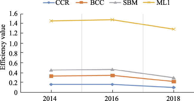
Fig. 1 Trends in farm productivity at the farm household level over the sample period
The above figure shows the overall level and trend of micro agricultural productivity of the sample farmers. From the mean results, the measurement results of different models differ slightly, the conclusions of the same model are generally consistent with the findings of the existing literature, showing the scientific and representative nature of the sample data, but in general, the agricultural productivity at the farmer level is relatively low, and there is still more room for improvement (Wang et al., 2020; Zhang et al., 2023), and from the time series, the change trends are generally the same within the sample period. This indicates that the model is accurate and basically matches the actual agricultural production, and can portray the changes of realistic agricultural productivity.
In terms of measurement type, the CCR model-based integrated technical efficiency value of farm households characterizes the product of pure technical efficiency and scale efficiency, which increased slightly from 0.1576 to 0.1592 from 2014 to 2016 in the sample period, and then declined significantly to 0.0964 in 2018, with a drop of 39.45%, much higher than the increase in the previous sample period, giving micro farm households comprehensive resource allocation and resource use efficiency measurement and evaluation provides a reference basis. The pure technical efficiency value of farm households based on the BCC model increased from 0.1754 in 2014 to 6.78% and reached 0.1873 in 2016, while it decreased as much as 33.9% to 0.1238 in 2018, which combined with the comprehensive technical efficiency value of farm households from the CCR model indicates that the scale efficiency of farm households did not change much during the sample period, confirming the established studies (Xu et al., 2011; Wang and Xin, 2022). In terms of the efficiency values for farm households based on the SBM model, the efficiency values of 2014, 2016, 2018 were 0.1242, 0.1239 and 0.0753, showing a decreasing trend year by year with an average annual decrease of 13.12%, implying that the average production efficiency of the sample farm households was decreasing when considering the slack inputs and slack outputs of farm households. And when incorporating the green total factor efficiency values measured by the technology-optimized Malmquist-Luenberger index, with 2014 as the base period, increased by 0.99% in 2016 and decreased by 0.4% in 2018, both in line with the national macro agricultural green total factor productivity (Ma and Tan, 2021), and replacing the non-expected output representation the results differ slightly after replacing the variables, but the overall trend and amount of change are roughly the same, implying that green agricultural development at the micro level still has a long way to go and deserves focused attention.

6 Conclusions

Accelerating the transformation and upgrading of agriculture and transforming from a large agricultural country to a strong agricultural country is the call of the times for the modernization of agriculture with Chinese characteristics, the improvement of agricultural production efficiency, especially the improvement of green total factor productivity, has become a top priority. As one of the important aspects of efficiency measurement, the measurement of micro-farm productivity has become a hot issue. The study conducts a comparative analysis of four measures of agricultural integrated technical efficiency, pure technical efficiency, efficiency level values and agricultural green total factor productivity at the micro-farmer level, and applies the appropriate methodology to the actual study. The main findings are as follows:
First, based on the same input-output data, the measurement comparison of different models found that although there are differences in the calculated efficiency values, the calculated results and change trends of these four models have a high degree of consistency. The efficiency value calculated by CCR is a weakly effective, and the pure technical efficiency value calculated by BCC is the main factor affecting the efficiency value of micro agricultural production at the farmer level. Compared with the traditional CCR and BCC models, the SBM model is based on the method of calculating efficiency values on slack variables and can measure the amount of improvement of each calculated variable, so the SBM model is to optimize the CCR and BCC models and is more suitable for the formulation and optimization of Chinese government policies.
Second, through a detailed comparison of the technically optimized Malmquist-Luenberger index method and the above three measures, it is found that there are significant differences in the estimation results of production efficiency, but there is a high degree of consistency in the ranking of sample farmers. Meanwhile, from further comparisons in terms of diverse and variable models, method applicability, negative output treatment and efficiency interpretation, the Malmquist-Luenberger index method based on technology optimization was found to be the preferred method for micro-agricultural production efficiency measurement, with the characteristics of diverse model selection, rich application scenarios and easy processing of negative outputs.
Third, after adding environmental variables and random noise, the agricultural green total factor productivity at the farmer level is significantly increased, indicating that environmental factors mainly play a negative inhibitory role, and this negative effect is generally greater among both the farmers with higher and higher ranking of green development and the relatively weaker micro samples. How to grasp the main line of agricultural green development, give full play to the advantages of agricultural green technological progress, optimize and improve the efficiency of agricultural green technology, and reduce the negative externality output of environmental variables has become one of the key issues facing the enhancement of green total factor production in the micro farmer layer at present.
Fourth, by comparing the two measurement methods of environmental non-expected output, from the comparison of the results of statistical tests, the measurement results of the subjective and objective measurement methods have both certain correlation and differences. From the comparison of the two measurement methods in terms of measurement methods, data processing and realization forms, the measurement results of the two measurement methods have both differences and certain correlation, which will remain an important way to measure environmental factors of agricultural green total factor productivity in the future, and can be used in practical applications according to the comprehensive choice of research purposes and data availability.
The efficiency issue is an important issue in agricultural production and a fundamental issue in building a strong agricultural country, the related research objects have been expanding, the research fields have been deepening, and the research methods have been improving. This paper compares and analyzes the possible reasons for model differences and indicator inconsistencies using four microscopic farm-level agricultural production efficiency measurement models and multiple groups of indicators measuring farm-level agricultural production efficiency based on common sample indicators, providing an all-round mirror for effective improvement of agricultural production efficiency. However, due to the limitations of data collection and the limitations of our own research level, the research in this paper is still in the exploratory stage relative to the research field of production efficiency, and there are still many shortcomings: First, due to the applicability of the model and the limited indicators of micro-farmers, there are few existing research results in the academic community, and there are not many references available, so as a micro-farmers level agricultural production efficiency measurement and comparison. Therefore, as a trial and exploration in the measurement and comparison of agricultural production efficiency at the microfarm level, there are still many immature points in the selection of indicators and the application of methods, which need to be further improved to enrich the measurement of micro agricultural production efficiency. Second, as an important branch of efficiency measurement, the Malmquist-Luenberger index model based on technical optimization can be further extended, and more breakthroughs need to be explored with specific application scenarios in the future. This is also the next direction to focus on.

Acknowledgement

We are grateful to the Soft Science Project of the Rural Revitalization Expert Advisory Committee of the Ministry of Agriculture and Rural Affairs, Central Agricultural Office, the Excellent Talents Support Project and the College Students Innovation and Entrepreneurship Training Program.
[1]
Aparicio J, Barbero J, Kapelko M, et al. 2017. Testing the consistency and feasibility of the standard Malmquist-Luenberger index: Environmental productivity in world air emissions. Journal of Environmental Management, 196(3): 148-160.

DOI

[2]
Banker R D, Charnes A, Cooper W W. 1984. Some models for estimating technical and scale inefficiencies in date envelopment analysis. Management Science, 30(9): 1078-1092.

DOI

[3]
Chari A V, Liu E, Wang S, et al. 2021. Property rights, land misallocation and agricultural efficiency in China. Review of Economic Studies, 88(4): 1831-1832.

DOI

[4]
Charnes A, Cooper W W, Rhodes E. 1978. Measuring the efficiency of decision making units. European Journal of Operational Research, 2(6): 429-444.

DOI

[5]
Cheng Y S. 2022. Research on the influence of agricultural socialization service on green total factor productivity: Based on the perspective of farmer household’s factor endowments. Diss., Hefei, China: Anhui University. (in Chinese)

[6]
Cheng Y S, Zhang D Y. 2022. Analysis of the impact of social insurance on farmers’ subjective well-being from the perspective of common prosperity and the mechanism: China’s experience and evidence. Frontiers in Psychology, (3): 1-16.

[7]
Cheng Y S, Zhang D Y, Wang X. 2022. Agricultural socialized services to promote green development: An analysis based on farmer households’ perspective. Resources Science, 44(9): 1848-1864. (in Chinese)

[8]
Cheng Y S, Zhang D Y, Wang X. 2023. Measurement and analysis of agricultural green total factor productivity based on farmers’ perspectives. Chinese Journal of Eco-Agriculture, 31(5): 820-834. (in Chinese)

[9]
Chung Y H, Färe R, Grosskopf S. 1997. Productivity and undesirable outputs: A directional distance function approach. Journal of Environmental Management, 51(3): 229-240.

DOI

[10]
Guo X M, Chen B Y, Wang K, et al. 2022. Measurement of total factor productivity and international comparison. Statistics & Decision, 38(12): 146-149. (in Chinese)

[11]
Huang S Y, Ma D C. 2021. Measurement and convergence analysis of total factor productivity of family forestry in Northwest China. Journal of Arid Land Resources and Environment, 35(2): 21-27. (in Chinese)

[12]
Li G C, Feng Z C, Fan L X. 2010. Is the small sized rural household more Efficient? The empirical evidence from Hubei Province. China Economic Quarterly, 9(1): 99-128. (in Chinese)

[13]
Li S M, Yin X W. 2017. Analysis of the impact of rural labor migration on total factor productivity in agriculture in China. Journal of Agrotechnical Economics, (9): 4-13. (in Chinese)

[14]
Liu M. 2020. Study on the influence and threshold effect of farm machinery input on green total factor productivity of agriculture. Diss., Changchun, China: Jilin Agricultural University. (in Chinese)

[15]
Ma G Q, Tan Y W. 2021. Impact of environmental regulation on agricultural green total factor productivity: Analysis based on the Panel Threshold Model. Journal of Agrotechnical Economics, (5): 77-92. (in Chinese)

[16]
Pan D, Ying R Y. 2013. Agricultural total factor productivity growth in China under the binding of resource and environment. Resources Science, 35(7): 1329-1338. (in Chinese)

[17]
Song J. 2021. Literature review of the impact of technological innovation on employment. Nanjing Business Review, (2): 60-88. (in Chinese)

[18]
Tone K. 2001. A slacks-based measure of efficiency in data envelopment analysis. European Journal of Operational Research, 130(3): 498-509.

DOI

[19]
Wang L, Yang R D, Wu B. 2020. A study on total factor productivity of agricultural production of rural households in China. Journal of Management World, 36(12): 94-110. (in Chinese)

[20]
Wang M Q, Wang J H, Zhao L M. 2017. A study on innovation drivers of family farms based on total factor productivity perspective: Empirical data from 228 family farms in Wuxi. Rural Economy, (5): 32-38. (in Chinese)

[21]
Wang Z, Xin X. 2022. Can cross-village land transfer achieve grain productivity growth? An empirical analysis based on rural household survey data from fifteen provinces. China Rural Survey, (2): 2-18. (in Chinese)

[22]
Xu Q, Yin R L, Zhang H. 2011. Economies of scale, returns to scale and the problem of optimum-scale farm management: An empirical study based on grain production in China. Economic Research Journal, (3): 59-71, 94. (in Chinese)

[23]
Zhang D B. 2018. Study on vegetable production efficiency by scale: Evidence from 2009-2016 surveys in main vegetable production areas. Journal of Agrotechnical Economics, (7): 41-50. (in Chinese)

[24]
Zhang M L, Tong T, Chen Z J. 2023. Can socialized service of agricultural production improve agricultural green productivity? South China Journal of Economics, (1): 135-152. (in Chinese)

[25]
Zhu S E, Yang R D, Wu B. 2018. Income mobility of rural households in China: 1986-2017. Journal of Management World, 34(10): 63-72. (in Chinese)

Outlines

/