
Journal of Resources and Ecology >
A Deep Learning-based Spatio-temporal NDVI Data Fusion Model
Received date: 2023-05-14
Accepted date: 2023-07-30
Online published: 2023-12-27
Supported by
The National Natural Science Foundation of China(31971507)
The National Natural Science Foundation of China(31861143015)
The Joint Research Project of the People’s Government of Qinghai Province and Chinese Academy of Sciences(LHZX-2020-07)
Satellite remote sensing provides the changes information of Earth surface on large spatial scale in a long time series and has been widely used in ecology. However, the possible impact from human activities generally occurs on a smaller spatial scale and could be detected in a longer time, which requires the remote sensing data having the both higher spatial and temporal resolution. Meanwhile, the development of the spatiotemporal data fusion algorithm provides an opportunity for the requirements. In this paper, based on deep learning, we proposed a residual convolutional neural network (Res-CNN) model to improve the fusion result considerably with brand-new network architecture to fuse the NDVI retrievals from Landsat 8 and MODIS images. Experiments conducted in two different areas demonstrate improvements by comparing them with existing algorithms. The model performance was evaluated by a linear regression between predictions and observations and quantified by determination coefficients (R2), regressive ecoefficiency (slope). The two excellent models, ESTARFM and FSDAF, were compared with the new model on their performance. The results showed that the predicted NDVI had the higher exploitational on the variability in the Landsat-based NDVI with the R2 of 0.768 and 0.807 at the urban and grassland sites. The predicted NDVI was well consistent with the observations with the slope of 1.01 and 0.989, and the R-RMSE of 95.76% and 93.58% at the urban and grassland sites respectively. This study demonstrated that the Res-CNN model developed in this paper exhibits higher accuracy and stronger robustness than the traditional models. This research is full implications because it not only provides a model on the spatio-temporal data fusion, but also can provide the data of a long time series for the management and utilization of agriculture and grassland ecosystems on the regional scale.
SUN Ziyu , OUYANG Xihuang , LI Hao , WANG Junbang . A Deep Learning-based Spatio-temporal NDVI Data Fusion Model[J]. Journal of Resources and Ecology, 2024 , 15(1) : 214 -226 . DOI: 10.5814/j.issn.1674-764x.2024.01.019
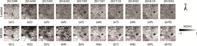
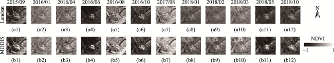
Table 1 The description on Daxing Dataset and AHB Dataset |
| Dataset | Image size | Pairs | Timespan |
|---|---|---|---|
| Daxing | 1640×1640 | 10 | 2013/09/01-2019/01/21 |
| AHB | 2800×2480 | 12 | 2015/09/25-2018/10/03 |
Table 2 Accuracy comparison of ablation experiments for Res-CNN model |
| Model | OA | F1-score |
|---|---|---|
| Res-CNN + Relu | 93.4% | 94.3% |
| Res-CNN + Mish | 96.3% | 97.3% |
Table 3 The quantitative evaluations on the fusion result on 29 April 2014 according to the Daxing Dataset |
| Daxing Dataset | Res-CNN | ESTARFM | FSDAF |
|---|---|---|---|
| RMSE | 1.09 | 1.28 | 1.34 |
| R2 | 0.768 | 0.737 | 0.658 |
| KGE | 0.78 | 0.695 | 0.745 |
| SSIM | 0.94 | 0.897 | 0.884 |
Table 4 The quantitative evaluations on the fusion result on 3 October 2018 according to the AHB dataset |
| AHB Dataset | Res-CNN | ESTARFM | FSDAF |
|---|---|---|---|
| RMSE | 1.06 | 0.93 | 0.983 |
| R2 | 0.807 | 0.764 | 0.786 |
| KGE | 0.898 | 0.867 | 0.888 |
| SSIM | 0.967 | 0.937 | 0.949 |
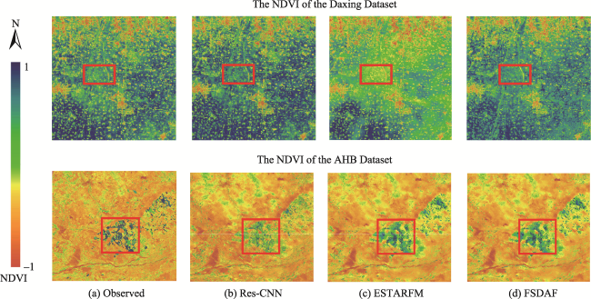
Fig. 9 The NDVI observation results of different methods in the Daxing area on April 29, 2016 and AHB Dataset on April 29, 2018. (a) Observed, (b) Res-CNN, (c) ESTARFM, (d) FSDAF |
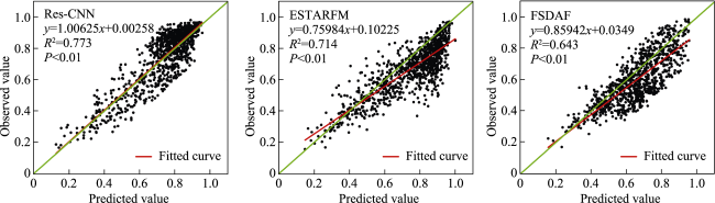
Fig. 10 The linear regression-based evaluation on the different data fusion models against the observed NDVI on April 29,2016 in the Daxing Data |
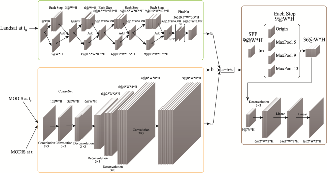
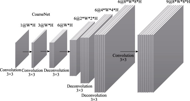
| Landsat t0 | MODIS t0 | MODIS t1 | |
|---|---|---|---|
| Inputs | 1024×1024 | 64×64 | 64×64 |
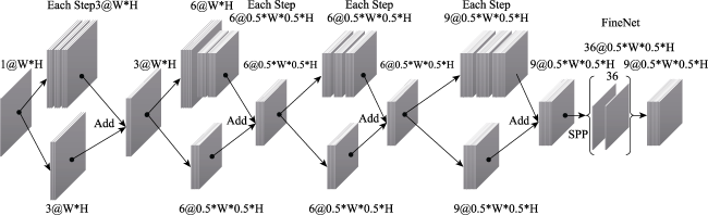
| Feature extraction | Res-Block 3×3 Conv2d Stride=1 1024×1024 | Two Layers 3×3 Conv2d Stride=1 64×64 | Two Layers 3×3 Conv2d Stride=1 64×64 |
| Res-Block 3×3 Conv2d Stride=2 512×512 | Three Layers 3×3 DeConv2d Stride=2 512×512 | Three Layers 3×3 DeConv2d Stride=2 512×512 | |
| Res-Block 3×3 Conv2d Stride=1 512×512 | 3×3 Conv2d Stride=1 512×512 | 3×3 Conv2d Stride=1 512×512 | |
| Res-Block 3×3 Conv2d Stride=1 512×512 | |||
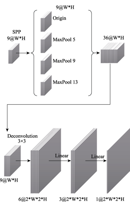
| SPP 512×512 | |||
| 3×3 Conv2d Stride=1 512×512 | |||
| Use a represent Landsat t0’s feature map | Use b represent MODIS t0’s feature map | Use c represent MODIS t1’s feature map | |
| Feature fusion | a‒b+c 512×512 | ||
| Feature reconstruction | 3×3 DeConv2d Stride=2×1024×1024 | ||
| FCN 1024×1024 | |||
| FCN 1024×1024 | |||
| [1] |
|
| [2] |
|
| [3] |
|
| [4] |
|
| [5] |
|
| [6] |
|
| [7] |
|
| [8] |
|
| [9] |
|
| [10] |
|
| [11] |
|
| [12] |
|
| [13] |
|
| [14] |
|
| [15] |
|
| [16] |
|
| [17] |
|
| [18] |
|
| [19] |
|
| [20] |
|
| [21] |
|
| [22] |
|
| [23] |
|
| [24] |
|
| [25] |
|
| [26] |
|
| [27] |
|
| [28] |
|
| [29] |
|
| [30] |
|
| [31] |
|
| [32] |
|
| [33] |
|
| [34] |
|
| [35] |
|
| [36] |
|
| [37] |
|
| [38] |
|
| [39] |
|
| [40] |
|
| [41] |
|
| [42] |
|
| [43] |
|
| [44] |
|
| [45] |
|
| [46] |
|
/
| 〈 |
|
〉 |