Impact of Human Activities on Ecosystem

The Ozone Concentration and Changes in the Sensitivity of Its Formation in Guangdong-Hong Kong-Macao Greater Bay Area (GBA) from a Carbon Neutral Perspective

  • HAO Jianghong , 1 ,
  • LI Yue , 2, * ,
  • ZHAO Ying 1 ,
  • CHENG Qinyu 1 ,
  • ZHAO Xiuyong 3 ,
  • CHEN Dongsheng 1
Expand
  • 1. Key Laboratory of Beijing on Regional Air Pollution Control, Faculty of Environment and Life, Beijing University of Technology, Beijing 100124, China
  • 2. Laboratory of Transport Pollution Control and Monitoring Technology, Transport Planning and Research Institute, Ministry of Transport, Beijing 100028, China
  • 3. State Key Laboratory for Clean and Efficient Coal-fired Power Generation and Pollution Control, National Environmental Protection Research Institute for Electric Power Limited Company, Nanjing 210031, China
*LI Yue, E-mail:

Received date: 2023-05-13

  Accepted date: 2023-07-23

  Online published: 2023-12-27

Supported by

The National Natural Science Foundation of China(51978011)

The Opening Project of State Key Laboratory for Clean and Efficient Coal-fired Power Generation and Pollution Control(D2022FK082)

Abstract

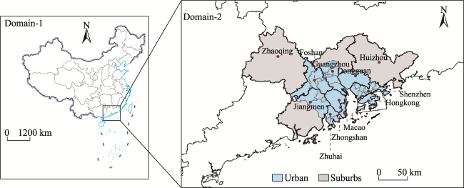
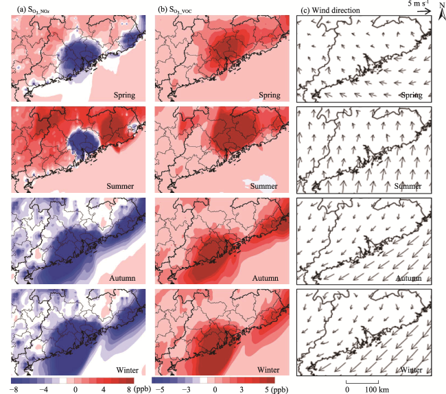
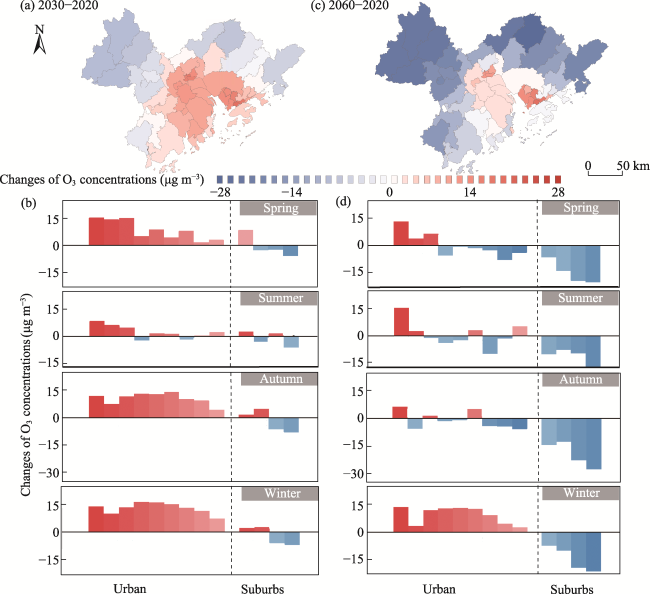
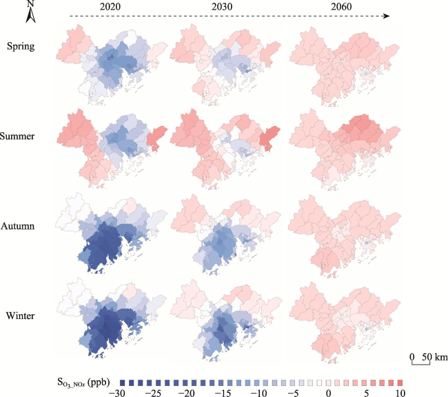
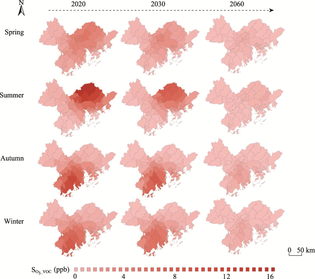
To investigate the potential impact of emission reduction measures on ozone (O3) formation under the carbon neutrality target, we examined the changes in O3 concentration and their sensitivity to various parameters in the urban and suburban areas of the Guangdong-Hong Kong-Macao Greater Bay Area (GBA). In this study, we used the Weather Research and Forecasting (WRF), the Sparse Matrix Operator Kernel Emissions (SMOKE) and the Community Multi-scale Air Quality Modeling system (CMAQ) air quality model to simulate O3 formation in three key years of 2020, 2030 and 2060, based on the Ambitious-pollution-Neutral-goal scenario data from the Dynamic Projection for Emissions in China (DPEC) model. The decoupled direct method (DDM) module embedded in CMAQ was used to calculate the first-order sensitivity coefficients of O3 to nitrogen oxides (SO3_NOx) and volatile organic compounds (SO3_VOC). The results show several important trends in the O3 concentrations and sensitivity. (1) For the changes in O3 concentrations, in terms of different seasons, the O3 concentration in the GBA region shows an increasing trend in winter in both 2030 and 2060 compared to 2020. In terms of different cities, the O3 concentration in Shenzhen shows a significant increasing trend compared to the other cities. (2) For changes in O3 sensitivity, SO3_NOx shows an increasing trend, with the negative area declining and the positive area increasing. In 2030, the negative absolute value of SO3_NOx is reduced, indicating that the NOx titration effect will be weakened. In 2060, SO3_NOx becomes positive in most areas of the GBA region. For SO3_VOC, the future scenario shows positive values throughout the study area for all years, but a decreasing trend.

Cite this article

HAO Jianghong , LI Yue , ZHAO Ying , CHENG Qinyu , ZHAO Xiuyong , CHEN Dongsheng . The Ozone Concentration and Changes in the Sensitivity of Its Formation in Guangdong-Hong Kong-Macao Greater Bay Area (GBA) from a Carbon Neutral Perspective[J]. Journal of Resources and Ecology, 2024 , 15(1) : 204 -213 . DOI: 10.5814/j.issn.1674-764x.2024.01.018

1 Introduction

The Guangdong-Hong Kong-Macao Greater Bay Area (GBA) is one of the most highly urbanized and industrialized regions in China, with a population of more than 50 million (Ma et al., 2007). The Gross Domestic Product (GDP) of the GBA has been growing rapidly and was estimated to be around 1.5 trillion USD in 2022 (http://www.cnbayarea.org.cn). It is expected to become one of the leading international bay areas and world-class urban agglomerations in the near future. However, the GBA has experienced severe photochemical smog pollution in recent years, and extremely high levels of surface ozone (O3) are frequently observed. This has adverse impacts on the human health and the ecological environment, limiting the sustainable development of the society and economy (Chen et al., 2020b). Therefore, reducing O3 pollution has become a major task for improving air quality over the GBA region.
Near-surface O3 is a secondary pollutant produced by a series of chemical reactions between precursors such as volatile organic compounds (VOC) and nitrogen oxides (NOx) (Haagen-Smit, 1952; Chameides et al., 1992). The relationship between O3 and its precursors exhibits complex non-linear features and is influenced by several factors (Wang et al., 2017). One of the most critical factors influencing the O3 level is the relative ratios of precursor species. Previous studies have generally classified the sensitivity of O3 to its precursors into VOC-sensitive, transitional, and NOx-sensitive regions based on differences in the response results (Chock and Heuss, 1987; Lu et al., 2019; Liu and Shi, 2021). In the different sensitivity regions, the variations in O3 concentrations due to reductions in the emissions of each precursor species are very different (Liu and Shi, 2021). In the VOC-sensitive region, O3 concentrations are highly sensitive to changes in VOC emissions and decrease as the VOC concentrations decrease. However, controlling NOx emissions may weaken the titration effect of NO, leading to a greater accumulation of O3 and causing an increase in O3 concentrations. In the NOx-sensitive region, O3 production is more dependent on NOx, where the O3 concentration decreases as NOx emissions are reduced. Meanwhile, changes in VOC emissions in these regions have minimal effect on O3 formation. In the transition region, O3 concentrations exhibit small changes with declining concentrations of both VOC and NOx. Therefore, the accurate determination of O3 sensitivity is a crucial prerequisite for the formulation of environmental management and emission control policies (Li et al., 2021).
At the 75th session of the United Nations General Assembly, China set the goal of achieving “peak carbon” by 2030 and “carbon neutrality” by 2060 (hereafter referred to as the “double carbon” goal). Many expect that China will continuously optimize its energy structure in the future to achieve this goal. These adjustments will inevitably lead to changes in the emission structure of pollutants (Wang, 2021), including the emissions and relative ratios of NOx and VOC (Zhu et al., 2021). As a result, O3 sensitivity is expected to change, posing new challenges for O3 pollution control (Jin and Holloway, 2015). As one of the most developed urban agglomerations in South China, the GBA exhibits significant differences in the emission structures between urban and suburban areas due to its high level of urbanization and frequent industrial and transportation activities. Therefore, conducting a comprehensive analysis of the future trends of O3 sensitivity and considering the urban-suburban differences are necessary in order to provide a reference for the scientific formulation of O3 pollution control strategies.
In this study, we used the Weather Research and Forecasting (WRF), the Sparse Matrix Operator Kernel Emissions (SMOKE) and the Community Multi-scale Air Quality Modeling system (CMAQ) to simulate O3 concentrations in three key years of 2020, 2030 and 2060, based on the emissions data from the Ambitious-pollution-Neutral-goal scenario, which were provided by the Dynamic Projection model for Emissions in China (DPEC). The sensitivities of O3 to its main precursors of NOx and VOC were calculated using the Decoupled Direct Method (DDM) module embedded in CMAQ. A comparative analysis of the spatial and temporal distribution changes in the urban and suburban of O3 concentrations and sensitivity between different years was conducted, with the aim of providing a decision-making basis for future O3 pollution prevention and control policies in the GBA region.

2 Methods

2.1 Study area

Figure 1 shows the map of the study area and two nested domains that were established for the modeling system. Domain 1 covers most of China, with a grid resolution of 27 km×27 km. Domain 2 covers the GBA region, with a grid resolution of 9 km×9 km (from 20.5°N to 24.8°N and 111.7°E to 116.3°E).
Fig. 1 Map of the study area and the locations of the urban and suburban areas
We considered the GBA as a whole region and identified the locations of the central urban areas according to the methodology of Zeng et al. (2022). Grids with population densities above the 99th percentile are defined as central urban areas, while the remainder of the area is considered suburban. The population density and GDP data were obtained from the GPW v4.11 dataset of the NASA Earth Observing System Data and Information System (https://sedac.ciesin.columbia.edu). We identified the urban and suburban distribution of the GBA region based on the above method and compared the identification results with those of other studies (Chen et al., 2020b), and the urban-suburban distribution shows a good consistency. In this study, southern Guangzhou, western Dongguan, Shenzhen, Foshan, eastern Jiangmen, Zhongshan, Zhuhai, Macao and Hong Kong were defined as the central urban areas of the GBA region, while all other places were defined as suburban areas. The specific results are shown in Fig. 1.

2.2 Input data and model configuration

In this study, we employed the WRF-SMOKE-CMAQ modeling system to predict future ozone formation changes in the GBA region. The configuring details and the input data of the modeling system are summarized as follows.
Meteorological data. We selected 2020 as the base year for meteorological data and maintained consistency with its conditions for 2030 and 2060. The meteorological field input file was derived from the Final Operational Model Global Analysis data (http://rda.ucar.edu/datasets/ds083.3) from the National Center for Environmental Prediction (NCEP), with a temporal resolution of 6 h and a spatial resolution of 0.25° × 0.25°.
Emission data. We chose the Ambitious-pollution-Neutral- goal scenario data (http://meicmodel.org/) from the Dynamic Projection model for Emissions in China (DPEC) (Cheng et al., 2021). The year of 2020 was selected as the base year and 2030 and 2060 were selected as the other target years for the simulations.
The WRF model configuration. Version 3.9 of the Weather Research and Forecasting (WRF) model was used to simulate meteorological conditions in this study. The model configurations for the WRF are shown in Table 1.
Table 1 Summary of WRF model configurations in this study
Category Detailed configuration
Microphysics scheme Purdue Lin
Shortwave radiation scheme New Goddard
Long-wave radiation scheme Rapid Radiative Transfer Model (RRTM)
Planetary Boundary Layer (PBL) scheme YSU
Land-Surface scheme Noah
Cumulus scheme Kain-Fritsch cumulus
The CMAQ model configuration. The CMAQv5.0.2 model was used in this study. The Carbon Bond-5 mechanism with the chlorine and updated toluene chemistry and sixth-generation CMAQ aerosol module, with extensions for sea salt emissions and thermodynamics, were selected as model configurations. The DDM module within the CMAQ model allows the simultaneous calculation of local sensitivities of pollutant concentrations to the input parameters. For the setting of the sensitivity input file we referred to Luecken et al. (2018). Each source category was tracked separately for NOx (sum of NO and NO2; and here we also added HONO when it is assumed to be a portion of the NOx emissions) and hydrocarbons (sum of model species Paraffin carbon bond PAR, Ethane (ETHA), Methanol (MEOH), Ethanol (ETOH), Formaldehyde (FORM), Acetaldehyde (ALD2), Propionaldehyde and higher aldehydes (ALDX), Ethene (ETHE), Terminal olefin carbon bond (OLE), Internal olefin carbon bond (IOLE), Isoprene (ISOP), Terpene (TERP), Toluene and other monoalkyl aromatics (TOL), and Xylene Aerosol (XYL)).
Like other AQMs, CMAQ numerically conserves and describes the formation and transport of air pollutants primarily by solving the advection-diffusion-reaction equations:
$\frac{\partial {{C}_{i}}}{\partial t}~$=$-\nabla \left( u{{C}_{i}} \right)$+$\nabla \left( K\nabla {{C}_{i}} \right)+{{R}_{i}}$$+~{{E}_{i}}$ $\left( i=1,2,\cdots,N \right)$
where Ci is the average concentration of species i at each grid cell, and u, K and N are the wind field, turbulent diffusivity tensor and number of chemical species, respectively. Ri and Ei represent the chemical reaction rates and emission rate of species i, respectively, and $\nabla $ represents the change of each variable within time t.
The first order sensitivity coefficient calculated by the DDM module is defined as:
$S_{ij}^{\left( 1 \right)}$=$\text{ }\!\!~\!\!\text{ }\frac{\partial {{C}_{i}}}{\partial {{p}_{j}}}$
where $S_{ij}^{\left( 1 \right)}$ is the first-order sensitivity coefficient of the CMAQ concentration field output species i relative to the sensitivity parameter pj. This coefficient depends on the magnitude of the sensitive parameter and does not provide a basis for comparison. Therefore, the first-order sensitivity coefficient Sij(1) was unified by applying the semi-normalization method, as shown in equation (3):
$S_{ij}^{\left( 1 \right)}$=${{\tilde{p}}_{j}}\text{ }\!\!~\!\!\text{ }\frac{\partial {{C}_{i}}}{\partial {{p}_{j}}}$=${{\tilde{p}}_{j}}\frac{\partial {{C}_{i}}}{\partial ({{\epsilon }_{j}}{{p}_{j~}})}$=$\frac{\partial {{C}_{i}}}{\partial {{\epsilon }_{j}}}$
Where ${{\tilde{p}}_{j}}$ is the unperturbed value, and ${{\epsilon }_{j}}$ is a scaling variable with a scalar of 1. By integrating equation (3) with respect to time t and substituting it into equation (1), we can derive the first-order sensitivity coefficient DDM equation, as shown in equation (4):
$\frac{\partial S_{ij}^{\left( 1 \right)}}{\partial t}$=$-\nabla \left( uS_{ij}^{\left( 1 \right)} \right)+\nabla \left( K\nabla S_{ij}^{\left( 1 \right)} \right)+{{J}_{i}}S_{j}^{\left( 1 \right)}+\frac{\partial {{R}_{i}}}{\partial {{\epsilon }_{j}}}{{\delta }_{5{{j}_{1}}}}+$
$\tilde{E}{{\delta }_{1{{j}_{1}}}}{{\delta }_{i{{j}_{2}}}}-\nabla (\tilde{u}{{C}_{i}})\ {{\delta }_{3{{j}_{1}}}}+\nabla \left( \tilde{K}\nabla {{C}_{i}} \right){{\delta }_{4{{j}_{1}}}}$
where ${{J}_{i}}$ is the i-th row vector of the reaction rate Jacobian matrix. Sj(1) is the vector of first-order coefficients of sensitivity parameter ${{p}_{j}}$, and ${{\delta }_{ij}}$ is the Kronecker $\delta $ response function. The subscript $\text{ }\!\!~\!\!\text{ }{{j}_{1}}$ represents the type of sensitivity parameter ${{p}_{j}}$, and the values from 0 to 6 represent the sensitivity parameters for initial conditions, emission rates, boundary conditions, wind fields, diffusion rates, reaction rate constants, and dry deposition, respectively (Hakami et al., 2003). This equation is commonly used to study how the atmospheric system responds when one or more elements change, and therefore can be used to calculate quantitative relationships between O3 and source emissions (Napelenok et al., 2008).

2.3 Model evaluation

The WRF model and the CMAQ model have been extensively applied and evaluated in our previous studies (Chen et al., 2017; Chen et al., 2020a; Chen et al., 2021) and in those of other researchers (Ye et al., 2016; Wang et al., 2019). In this study, similar indicators were used to evaluate the model performance for the base year (2020), including the values of the Mean Bias (MB), Mean Absolute Error (MAE), Normalized Mean Bias (NMB), Mean Fractional Bias (MFB), and correlation coefficient (R).
To evaluate the performance of the WRF model, Table 1 shows the comparison of simulated and observed meteorological parameters (http://data.cma.cn/) at 75 meteorological stations located in the study area in each simulated season of 2020, including temperature at 2 m (T2), relative humidity at 2 m (RH2) and wind speed at 10 m (WS10). To evaluate the performance of the CMAQ model, Table 2 shows the comparison of simulated and observed O3 concentrations for the 57 representative cities (http://www.cnemc.cn/) in each simulated season of 2020.
Table 2 Statistics for temperature at 2 m (T2), relative humidity at 2 m (RH2), and O3 concentration in 2020
Statistical indicator Season MBa MAEb NMBc (%) MFBd (%) Re
T2 (℃) Spring -2.2 3.1 -29.3 -21.3 0.8
Summer 2.1 3.4 11.6 9.75 0.8
Autumn 0.1 2.0 -8.2 29.8 0.9
Winter -1.2 3.0 -11.9 6.9 0.7
RH2 (%) Spring 2.2 9.3 14.9 2.8 0.7
Summer 7.8 15.5 25.7 12.6 0.7
Autumn -1.7 11.5 1.1 -4.4 0.6
Winter 2.1 15.3 6.7 1.8 0.6
O3 (μg m-3) Spring -5.9 15.7 8.0 15.3 0.7
Summer -3.5 19.8 0.1 9.3 0.8
Autumn -4.2 13.8 -0.5 1.2 0.8
Winter -6.7 9.7 13.3 22.5 0.7

Note: a, MB indicates the mean bias. b, MAE indicates the mean absolute error. c, NMB indicates the normalized mean bias. d, MFB indicates the normalized mean error. e, R indicates the correlative coefficient.

The results show high correlation coefficients (0.7≤R≤ 0.9), and low values for normalized mean bias and mean fractional bias (the absolute value≤30%) between the observed and simulated data, proving that the model performance was acceptable.

3 Results and discussion

3.1 Base year scenario

Figure 2 presents the seasonal spatial distribution of the first-order sensitivity coefficients of O3 to NOx (SO3_NOx) and VOC (SO3_VOC) as obtained from the CMAQ-DDM model. These coefficients represent the extent to which O3 concentrations respond to changes in the NOx and VOC emissions. For example, a positive SO3_NOx represents a positive correlation between O3 and NOx, i.e., O3 decreases as the NOx concentration decreases; and a negative SO3_NOx coefficient represents a negative correlation between O3 and NOx, i.e., O3 increases as the NOx concentration decreases. The meaning of SO3_VOC is similar. A higher absolute value of the first order sensitivity coefficient represents a more pronounced response of O3 to the precursors. In Fig. 2, positive first-order sensitivity coefficients are represented in red, while negative values are represented by blue. In Fig. 2a, the intensity of the blue represents the absolute value of the negative sensitivity coefficient for SO3_NOx, with darker blue representing a larger absolute negative value, which indicates a stronger titration effect of NOx.
Fig. 2 Seasonal first-order sensitivity coefficients of surface O3 to NOx (a) and VOC (b), and mean seasonal wind directions (c) in 2020 over the study area
As shown in Fig. 2, the urban O3 concentrations of the GBA region exhibit a higher sensitivity to changes in NOx and VOC emissions compared to suburban areas throughout all four seasons. It is particularly important to note that the central urban areas of the GBA region have a strong NOx titration effect. This is mainly due to the proximity of these areas to the ports, where the developed maritime transportation promotes extensive industrial and transportation activities, resulting in higher NOx emissions. The central urban areas of GBA are influenced by plumes rich in NOx, which strengthens the inhibitory effect of NOx on O3 formation. Additionally, the higher building density in the urban central areas also contributes to the higher O3 sensitivity to NOx and VOC emissions, as pollutants are more likely to accumulate in these areas, rather than being diluted as in the suburban regions. Therefore, urban planners need to implement effective measures to reduce vehicle emissions and industrial activities, and strengthen the management of urban central areas in order to protect the health of city residents and maintain environmental quality.
There is a clear seasonal variation in O3 sensitivity. SO3_VOC is positive throughout the year and is highest in summer (Fig. 2b). In contrast, SO3_NOx is negative most of the time and the range of negative regions is greater in autumn and winter than in spring and summer. This is mainly due to the dual role of NOx in the formation of O3 by modulating the chemistry of HOx radicals (Lu et al., 2019). In autumn and winter, the lower temperatures result in reduced volatility of VOC, while the NOx/VOC ratio increases, making the VOC cycle weaker compared to the NOx cycle. This leads to a stronger titration effect of NO on O3, resulting in negative values of SO3_NOx in most areas of the GBA region. Conversely, higher temperatures in spring and summer lead to greater volatility of VOC, resulting in lower NOx/VOC ratios, making the NOx cycle weaker relative to the VOC cycle. This results in some areas being limited by the strength of the NOx cycle and the consequent conversion of SO3_NOx to positive values. In addition, the high temperatures and strong solar radiation in summer provide suitable conditions for photochemical reactions, which make the SO3_VOC highest in summer.
O3 sensitivity is also influenced by various meteorological factors, one of which is wind direction. The influence of wind direction on O3 sensitivity in the GBA is particularly significant. Depending on the wind directions in different seasons (Fig. 2c), areas of negative SO3_NOx and areas of high SO3_VOC values extend downwind of these more developed industrialized cities. Therefore, when considering emission reduction measures in the GBA region, it is important to focus not only on the impact of NOx and VOC emissions, but meteorological factors such as wind direction should be considered.

3.2 Future scenarios

3.2.1 Trends in ozone concentrations

Figure 3a shows the annual average changes in the O3 concentrations in different counties of the GBA region in 2030. The values shown in the figure represent the differences in O3 concentrations between 2030 and 2020. The changes in O3 concentrations in urban and suburban areas show different results, with O3 concentrations in urban areas increasing by 8.6 μg m-3 and O3 concentrations in suburban areas decreasing by 1.4 μg m-3. This difference is mainly due to the stronger NOx titration in the central urban area, where the reduction in NOx will lead to an increase in O3 concentrations. Figure 3b shows the changes in O3 concentrations in the GBA area for the different seasons, where blue represents a decrease and red represents an increase. For the central city, the increases in O3 concentrations compared to 2020 are most pronounced in autumn (4.4-13.9 μg m-3) and winter (7.3-16.4 μg m-3). As mentioned in section of 3.1, the NOx titration is stronger in autumn and winter, so further research into the synergistic NOx and VOC reduction measures is needed. For the suburban areas, compared to 2020, the O3 concentration in Zhaoqing decreased most significantly, with reductions of 5.8-7.9 μg m-3. This is because SO3_NOx is positive in this area, and NOx emission reduction will cause the O3 concentration to decline, playing a superimposed role with the reduced O3 concentration caused by VOC emission reduction, resulting in a larger decrease in the O3 concentration.
Fig. 3 Annual and seasonal changes in MDA8 O3 concentrations in 2030 (a) & (b) and 2060 (c) & (d)

Note: In the column charts of (b) and (d), the cities of the urban category from left to right are: Shenzhen, Dongguan, Guangzhou, Jiangmen, Zhongshan, Macao, Foshan, Zhuhai, and Hong Kong, and the cities of the suburbs from left to right are: Guangzhou, Jiangmen, Huizhou and Zhaoqing.

Figure 3c shows the changes in annual average O3 concentrations in the different districts and counties in the GBA region in 2060. The values shown in the figure are the differences in O3 concentrations between 2060 and 2020. The O3 concentration in the central city of the GBA region increases by 1.9 μg m-3 while in the suburbs it decreases by 15.0 μg m-3. The changes in O3 concentrations in the GBA region in different seasons are shown in Fig. 3d. Note that the O3 concentrations in Shenzhen show an increasing trend for all seasons, ranging from 6.3 to 15.7 μg m-3, and therefore further research on O3 pollution control policies in this city is needed.
Overall, in terms of the different seasons, the O3 concentrations of the urban area in winter show increasing trends in both 2030 and 2060. These results suggest that for the GBA region, it may be necessary to make winter the key prevention and control period in the future ozone pollution control strategy. In terms of different cities, the O3 concentrations in Shenzhen show a significant upward trend compared to the other cities. Therefore, further research on the synergistic emission reduction strategy in Shenzhen is needed.

3.2.2 Trends in ozone sensitivity

Figure 4 shows the seasonal variations of SO3_NOx for 2020, 2030 and 2060 in the GBA region. The future scenarios show reductions in the absolute negative SO3_NOx values, indicating a weakening of NOx titration in 2030 compared to the status quo. At that point, the NOx reduction will still lead to an increase in O3 concentrations, but the reduced absolute negative values of SO3_NOx and the weakening of the NOx titration will result in smaller increases in O3 concentrations for the same percentage of NOx reduction. Compared to suburban areas, urban areas have a stronger NOx titration effect, and this spatial distribution will lead to a greater increase in O3 concentrations in urban areas than in suburban areas. Due to future urbanization policies, the urban population will increase and the increase in O3 concentrations in central urban areas will pose a greater health risk. By 2060 there will be a positive SO3_NOx conversion for most of the GBA, suggesting that reducing the NOx emissions after 2060 will have a positive effect on controlling O3 pollution, thus reducing the complexity of the O3 management problem.
Fig. 4 Spatial distributions of first-order sensitivity coefficients of surface O3 to NOx in different seasons in 2020, 2030 and 2060
Figure 5 shows the seasonal variations of SO3_VOC in 2020, 2030 and 2060. Compared to the status quo in 2020, the SO3_VOC will continue to decline in the future. The spatial distributions of SO3_VOC in all seasons in 2030 are approximately the same as in 2020, but the overall values are smaller. Specifically, the regional mean SO3_VOC in the GBA region declines from 3.0 ppb in 2020 to 1.8 ppb in 2030 in the spring, from 4.5 ppb to 2.8 ppb in the summer, from 4.1 ppb to 2.9 ppb in the autumn and from 3.6 ppb to 2.7 ppb in the winter. The values of SO3_VOC fall to lower levels (0-2 ppb) throughout 2060, suggesting that in 2060, the VOC reductions will result in a relatively small reduction in O3 concentrations. However, the results of SO3_NOx in 2060 show that SO3_NOx will be converted to positive values in most of the GBA, at which point NOx reductions will lead to a reduction in the O3 concentrations; and they will be superimposed on the reduction in O3 concentrations from VOC reductions, leading to a rapid decline in O3 concentrations.
Fig. 5 Spatial distributions of first-order sensitivity coefficients of surface O3 to VOC in different seasons in 2020, 2030 and 2060

4 Conclusions

In this study, the WRF-SMOKE-CMAQ-DDM air quality model was used to simulate O3 concentrations for the GBA region in three key years of 2020, 2030 and 2060, based on the emission data of the Ambitious-pollution-Neutral-goal scenario provided by the DPEC model for China’s future emissions. The sensitivity of O3 to precursors was investigated using the DDM module embedded in CMAQ. On this basis, this study investigated the urban and suburban spatial distribution patterns of the current and future O3 concentrations and their sensitivity in the GBA region, and provides a comparative analysis of the changes between different years. The main conclusions can be divided into the base year and future scenarios.
Base year scenario: The results of the DDM calculations for all seasons in the GBA region show that O3 concentrations are more responsive to changes in NOx and VOC emissions in urban areas compared to suburban areas. Notably, the central urban area shows larger negative absolute values of SO3_NOx, indicating a stronger NOx titration effect compared to the suburban areas. The spatial distribution of SO3_NOx varies between seasons, with larger areas of negative values in autumn and winter than in spring and summer. The values of SO3_VOC are positive throughout the year and the highest values occur in summer. The sensitivity of O3 formation in the GBA is strongly affected by wind direction. The negative areas of SO3_NOx and the areas of high values of SO3_VOC are influenced by the wind direction in different seasons, and extend downwind of these more developed industrialized cities.
Future scenario: 1) Regarding the changes in O3 concentrations, in terms of the different seasons, the GBA region shows an increasing trend in the urban winter O3 concentrations in both 2030 and 2060 compared to 2020. It is likely that winter will be the key period for prevention and control in the future ozone pollution control strategy. In terms of the different cities, the O3 concentrations in Shenzhen show a significant upward trend compared to the other cities. Therefore, further research on the synergistic emission reduction strategy in Shenzhen is needed. 2) Regarding the changes in O3 sensitivity, the overall trend of SO3_NOx is increasing, with the area of negative values decreasing and the area of positive values expanding. In 2030, the absolute value of the negative SO3_NOx decreases and the NOx titration effect is weakened. In 2060, SO3_NOx is transformed into positive values in most areas of the GBA, which suggests that the reduction of NOx emissions after 2060 will have a positive effect on controlling O3 pollution, and this could reduce the complexity of the O3 management issues. For SO3_VOC, the future scenario shows positive values for all years and an overall decreasing trend in the study area.
[1]
Chameides W L, Fehsenfeld F, Rodgers M O, et al. 1992. Ozone precursor relationship in the ambient atmosphere. Journal of Geophysical Research, 97(D5): 6037-6055.

DOI

[2]
Chen D S, Fu X Y, Guo X R, et al. 2020a. The impact of ship emissions on nitrogen and sulfur deposition in China. Science of the Total Environment, 708: 134636. DOI: 10.1016/j.scitotenv.2019.134636.

[3]
Chen D S, Wang X T, Li Y, et al. 2017. High-spatiotemporal-resolution ship emission inventory of China based on AIS data in 2014. Science of the Total Environment, 609: 776-787.

DOI

[4]
Chen D S, Xia L, Guo X R, et al. 2021. Impact of inter-annual meteorological variation from 2001 to 2015 on the contribution of regional transport to PM2.5 in Beijing, China. Atmospheric Environment, 260: 118545. DOI: 10.1016/j.atmosenv.2021.118545.

[5]
Chen Y, Yan H, Yao Y, et al. 2020b. Relationships of ozone formation sensitivity with precursors emissions, meteorology and land use types, in Guangdong-Hong Kong-Macao Greater Bay Area, China. Journal of Environmental Science, 94: 1-13. (in Chinese)

[6]
Cheng J, Tong D, Zhang Q, et al. 2021. Pathways of China’s PM2.5 air quality 2015-2060 in the context of carbon neutrality. National Science Review, 8: 63-73.

[7]
Chock D, Heuss J. 1987. Urban ozone and its precursors. Environmental Science & Technology, 21: 1146-1153.

DOI

[8]
Luecken D J, Napelenok S L, Strum M, et al. 2018. Sensitivity of ambient atmospheric formaldehyde and ozone to precursor species and source types across the United States. Environmental Science & Technology, 52: 4668-4675.

DOI

[9]
Haagen-Smit A J. 1952. Chemistry and physiology of Los Angeles Smog. Industrial & Engineering Chemistry, 44: 1342-1346.

DOI

[10]
Hakami A, Odman M T, Russell A G. 2003. High-order, direct sensitivity analysis of multidimensional air quality models. Environmental Science & Technology, 37: 2442-2452.

DOI

[11]
Jin X, Holloway T. 2015. Spatial and temporal variability of ozone sensitivity over China observed from the ozone monitoring instrument. Journal of Geophysical Research: Atmospheres, 120: 7229-7246.

[12]
Li D R, Wang S S, Xue R B, et al. 2021. OMI-observed HCHO in Shanghai, China, during 2010-2019 and ozone sensitivity inferred by an improved HCHO/NO2 ratio. Atmospheric Chemistry and Physics, 21: 15447-15460.

[13]
Liu C Q, Shi K. 2021. A review on methodology in O3-NOx-VOC sensitivity study. Environmental Pollution, 291: 118249. DOI: 10.1016/j.envpol.2021.118249.

[14]
Lu H, Lyu X, Cheng H, et al. 2019. Overview on the spatial-temporal characteristics of the ozone formation regime in China. Environmental Science Process & Impacts, 21: 916-929.

[15]
Ma X L, Tao L B H, Ma Y Y. 2007. Regarding the institutional innovation opportunity of Guangdong-Hong Kong regional environmental management from the perspective of the emission trading pilot scheme for thermal power plants in the Pearl River Delta region. Electric Power Technology and Environmental Protection, 90: 6-11. (in Chinese)

[16]
Napelenok S L, Cohan D S, Odman M T, et al. 2008. Extension and evaluation of sensitivity analysis capabilities in a photochemical model. Environmental Modelling & Software, 23: 994-999.

[17]
Wang N, Lyu X, Deng X, et al. 2019. Aggravating O3 pollution due to NOx emission control in eastern China. Science of the Total Environment, 677: 732-744.

DOI

[18]
Wang T, Xue L, Brimblecombe P, et al. 2017. Ozone pollution in China: A review of concentrations, meteorological influences, chemical precursors, and effects. Science of the Total Environment, 575: 1582-1596.

DOI

[19]
Wang Z X. 2021. Research on the pathway and policy framework of achieving carbon peak and carbon neutrality. Electric Power Technology and Environmental Protection, 37: 1-8. (in Chinese)

[20]
Ye L, Wang X, Fan S, et al. 2016. Photochemical indicators of ozone sensitivity: Application in the Pearl River Delta, China. Frontiers of Environmental Science & Engineering, 10(6): 49-62.

[21]
Zeng X R, Gao Y, Wang Y H, et al. 2022. Characterizing the distinct modulation of future emissions on summer ozone concentrations between urban and rural areas over China. Science of the Total Environment, 820: 153324. DOI: 10.1016/j.scitotenv.2022.153324.

[22]
Zhu F H, Wang Y S, Xu Z, et al. 2021. Research on the development path of carbon peak and carbon neutrality in China’s Power Industry. Electric Power Technology and Environmental Protection, 37: 9-16. (in Chinese)

Outlines

/