Impact of Human Activities on Ecosystem

Assessing Soil Erosion Susceptibility Using Revised Morgan-Morgan-Finney Model: A Case Study from Kulekhani Watershed, Makawanpur, Nepal

  • THAPA Rabin , 1 ,
  • JOSHI Rajeev , 2, * ,
  • BHATTA Binod 1 ,
  • GHIMIRE Santosh 1
Expand
  • 1. Faculty of Forestry, Agriculture and Forestry University, Hetauda 44107, Nepal
  • 2. College of Natural Resource Management, Faculty of Forestry, Agriculture and Forestry University, Udayapur, Katari 56310, Nepal
*JOSHI Rajeev, E-mail:

Received date: 2023-08-16

  Accepted date: 2023-10-16

  Online published: 2023-12-27

Abstract

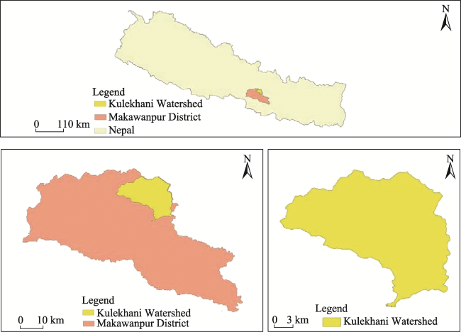
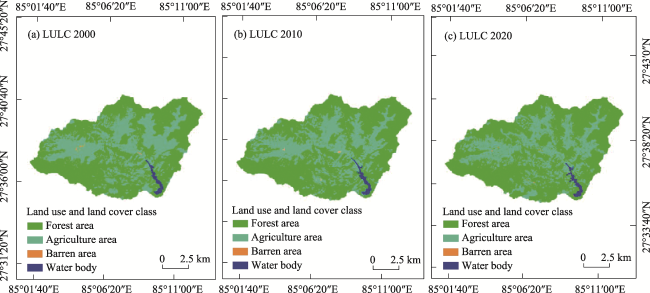
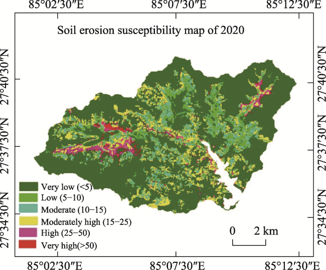
The research was conducted within the Kulekhani Watershed with the objective of examining changes in Land Use Land Cover (LULC) dynamics and soil erosion across various LULC categories spanning from 2000 to 2020. The findings regarding the LULC classification in the Kulekhani Watershed revealed a steady rise in forested land, escalating from 60.72% in 2000 to 62.43% in 2010, and ultimately reaching 64.75% of the total area by 2020. The extent of water bodies exhibited a marginal increase from 1.07% in 2000 to 1.08% in 2020. Correspondingly, barren land expanded from 0.21% to 0.26%, eventually reaching 0.35% over the successive time intervals. Conversely, agricultural land dwindled over these periods, comprising 38% in 2000, 36.24% in 2010, and ultimately declining to 33.82% by 2020. The utilization of the Revised Morgan-Morgan-Finney (RMMF) model for soil loss estimation demonstrated a declining trend in weighted average soil loss during the years 2000 to 2010, followed by a slight increase between 2010 and 2020. The calculated soil loss values were recorded as 8.64 t ha-1 yr-1, 7.12 t ha-1 yr-1, and 7.30 t ha-1 yr-1 for the years 2000, 2010, and 2020 respectively. Similarly, the erosion susceptibility map illustrated a rising pattern in the very low-risk soil erosion zone from 2000 to 2020, primarily prominent within forested regions, while exhibiting a low to moderate susceptibility in agricultural zones. Moreover, barren areas displayed a moderate to high susceptibility to soil erosion. To address these concerns, future endeavors are recommended to encompass afforestation initiatives in barren regions, implement conservation farming practices in agricultural areas, and adopt appropriate measures for road stabilization.

Cite this article

THAPA Rabin , JOSHI Rajeev , BHATTA Binod , GHIMIRE Santosh . Assessing Soil Erosion Susceptibility Using Revised Morgan-Morgan-Finney Model: A Case Study from Kulekhani Watershed, Makawanpur, Nepal[J]. Journal of Resources and Ecology, 2024 , 15(1) : 182 -196 . DOI: 10.5814/j.issn.1674-764x.2024.01.016

1 Introduction

Soil erosion embodies a natural mechanism entailing the removal and movement of soil materials, driven by erosive agents encompassing water, wind, gravity, and human activities (Aksoy et al., 2009). This phenomenon has garnered recognition as a foremost concern, with the Food and Agriculture Organization categorizing it among the ten principal threats to soil integrity, underscoring that the equivalent of a soccer field’s expanse of soil is eroded every five seconds. (FAO, 2015). Its implications are far-reaching, posing a substantial hazard to soil health, ecological equilibrium, and human well-being, as the lasting productivity of soil is significantly hampered by the disintegration and depletion of organic and topsoil components (Garcia-Ruiz et al., 2017). The repercussions extend to the exacerbation of events like landslides, riverbank collapses, floods, and droughts, with the escalating intensity and frequency of precipitation events attributed to climate change exacerbating the situation (Li et al., 2011).
In Nepal, a country characterized by its mountainous terrain, dynamic tectonics, and concentrated monsoon rains from June to September, a susceptibility to diverse natural hazards including landslides and soil erosion prevails (Chalise et al., 2019). Notably, water-induced soil erosion bears paramount significance due to its adverse ramifications for soil quality, aquatic ecosystems, and reservoir capacities. Several research investigations underscore the substantial magnitude of soil loss in Nepal, varying from negligible levels in lowlands to strikingly high rates of up to 105 Mg ha-1 yr-1 in upland regions and, at times, reaching an alarming 420 Mg ha-1 yr-1 in shrublands, primarily attributable to steep inclines, overgrazing, and improper land utilization (Bajracharya et al., 2009). Illustratively, annual soil erosion figures amount to approximately 75.83 t ha-1 in the Bagmati Basin, 64 t ha-1 in the Khajuri Catchment, 11.17 t ha-1 in Aringale Khola, and 14.7 t ha-1 in the Phewa Watershed of Nepal (Bastola et al., 2019; Chalise et al., 2019).
Soil loss from a specific landscape is shaped by a confluence of natural elements, encompassing intense rainfall, steep gradients, and fragile geological conditions, along with human-induced factors like overgrazing, unsustainable farming practices, excessive chemical input usage, and deforestation (Chalise et al., 2019). While the dominant contribution to erosion in Nepal arises from natural forces, the discernible imprint of human influence on soil erosion is undeniable (Shrestha et al., 2004). The onset of heavy pre-monsoon rainfall, accompanied by high-speed winds and hailstorms, amplifies the challenges of soil erosion, particularly within rain-fed agriculture (Atreya et al., 2006). Additionally, Land Use/Cover Change (LUCC) assumes a pivotal role as a determinant influencing soil erosion in landscapes, with the interplay of LUCC, atmospheric conditions, and topography exacerbating phenomena such as acidification, alkalization, soil erosion, and nutrient leaching (Li et al., 2014). Insightfully scrutinizing the dynamics of Land Use Land Cover (LULC) serves to elucidate the prevailing soil erosion dynamics and land vulnerability, thus providing a basis for future planning endeavors (Persichillo et al., 2017; Abdulkareem et al., 2019). Furthermore, Pradhan et al. (2012) underscore the potential to mitigate soil erosion by strategic adjustments, including modifications to LULC. Chalise et al. (2019) conducted a comprehensive analysis of LULC within the Sarada, Rapti, and Thuli Bheri river basins from 1995 to 2015, revealing a decline in forest and water body areas concurrent with an expansion of agricultural and built-up areas, culminating in an escalation of the erosion rate from 5.35 to 6.03 t ha-1 yr-1. To predict soil loss and assess erosion risk, a range of models is available, with the integrated use of satellite Remote Sensing (RS) and Geographic Information Systems (GIS) standing out as a highly effective approach for modeling erosional soil loss, integrating data on soil characteristics, LULC, terrain attributes, and meteorological inputs (Regmi et al., 2014).
This study employed the Revised Morgan-Morgan-Finney (RMMF) model to quantify the annual rate of soil erosion. The selection of this model was motivated by its straightforwardness, adaptability, and more robust physical foundation in comparison to the Universal Soil Loss Equation (USLE). Furthermore, it operates on a physically grounded empirical basis and necessitates fewer data inputs compared to most alternative erosion predictive models (Morgan et al., 1984). The model encompasses two distinct phases—water phase and sediment phase—to estimate soil erosion dynamics (Efthimiou, 2019). Soil erosion poses challenges to the effective utilization of natural resources and the livelihoods of communities (Tiwari et al., 2009). The ongoing decline in agricultural field productivity due to topsoil loss from erosion, coupled with increasing migration and the absence of young people for the stewardship of agricultural terraces, accentuates the predicament. Furthermore, the area’s vulnerability to soil erosion has been compounded by unregulated road construction and unpredictable climatic patterns, including intensified rainfall attributed to climate change (Schwilch et al., 2017). Since 1978, the Kulekhani Watershed has witnessed the implementation of soil conservation initiatives, encompassing measures such as conservation ponds, afforestation, road slope stabilization, torrent control, and gully and landslide stabilization (DSCWM, 2015). To establish a viable and sustainable watershed management framework, an assessment of the watershed’s condition, existing land use and land cover is indispensable, alongside the comprehensive characterization of present soil erosion status. This entails an evaluation of the current state of land use and land cover, predictions of future scenarios, and the thorough delineation of both current and projected soil erosion conditions. Notably, effective terrace management and traditional irrigation systems assume a pivotal role in ameliorating sediment generation and transport. The present study aims to employ geospatial tools of RS and GIS to analyze and model Land Use Land Cover (LULC) changes, evaluate the impact of these changes on soil erosion in the Kulekhani Watershed, making soil loss assessment of the reservoir catchment vital for its long-term conservation. The overarching goal is to assess soil erosion susceptibility using the Revised Morgan-Morgan-Finney model, with specific objectives including the analysis of LULC changes from 2000 to 2020 and the estimation of soil erosion within various LULC contexts.

2 Materials and methods

2.1 Study area

The Kulekhani Watershed Area (KWA) is situated within the Bagmati River Basin (BRB) of Makawanpur District and is positioned approximately 50 km southwest of the capital city, Kathmandu (Fig. 1). This watershed spans a geographical range of roughly 27°30′00″N to 27°40′46″N latitude and 85°01′41″E to 85°13′56″E longitude. It is subdivided into ten primary sub-watersheds, all of which contribute inflows to the 7-km long 114-meter- high rock fill dam that serves as a water source for downstream hydropower generation (Nippon, 1983). The Kulekhani River’s natural runoff at the dam site registers as low as 2.1 m3 s-1 during dry months and increases to 6.2 m3 s-1 during wet months (Shrestha et al., 2014). Consequently, the excess runoff during wet periods is stored in the reservoir to ensure consistent power generation during drier months. The Kulekhani Reservoir boasts an overall storage capacity of 85.3 million m3 (Schreier et al., 1995).
Fig. 1 Map of Kulekhani Watershed in Nepal
Kulekhani Watershed comprising steep hills and narrow valleys has uneven terrain (Pokharel and Thapa, 2018). The slope of the watershed ranges from 0° to 68.95° and elevation ranges from 1362 m to 2595 m at the dam site and the peak of Simbhanjyang of the Mahabharat range respectively (Fig. 2). The climate of Kulekhani Watershed varies from subtropical at lowlands to temperate at higher altitudes. It is under the influence of two major climatic zones namely warm temperate humid zone and cool temperate humid zone, which are mostly found in between the altitude 1500 m to 2000 m and above 2000 m respectively (Shrestha et al., 2014). The average annual precipitation over the watershed is about 1500 mm (Dhakal, 2011). The maximum and minimum daily temperature of the Kulekhani Watershed according to the temperature data from Department of Hydrology and Meteorology is 35 ℃ and -4.75 ℃ respectively. Kulekhani Watershed is in the Kathmandu complex of the lower Himalaya. The Kathmandu complex is divided into the Bhimphedi group and Phulchauki group separated. by a disconformity (Subedi and Acharya, 2016). The Kulekhani formation is a well-bedded alteration of the biotic schist and micaceous quartzite of dark and light as well as green and grey colours. Rockslides observed around Phedigaon were located on the schist of the Kulekhani formation (Sangroula, 2005).
Fig. 2 Altitudinal zone map and slope map of Kulekhani Watershed

2.2 Data used and methodology

2.2.1 Data sources

Primary data were gathered through on-site observation, satellite imagery, and topographical maps. Verification of information was conducted by comparing it with ground truth data obtained during fieldwork. Secondary data were sourced from various materials, including maps, reports, datasets, journals, and satellite images. The achievement of objectives was facilitated through the utilization of satellite data and supplementary information. The analysis of land use/land cover employed digital Landsat satellite data, boasting a resolution of 30 m. The creation of the land use/ cover change (LUCC) map was executed using the Google Earth Engine Platform. The annual report from the Department of Soil Conservation and Watershed Management, as well as soil maps and plant parameters from LRMP (1986) and Morgan (2001), were procured. Meteorological data were acquired from the Department of Hydrology and Meteorology.

2.2.2 Methods

The overall flow chart of the methodology used in this research is presented in Fig. 3.
Fig. 3 Flow chart of overall methodology
(1) Pre-fieldwork
The activities which were conducted in this stage were literature review and collection of secondary data, imagery and develop the base map.
Spatial data base generation: The soil, slope, and base maps were created by GIS processing. Following steps was followed for the database generation:
Creation of spatial data: Software, such as Arc GIS 10.8 and ILWIS 3.3 academic was used for creating spatial data, geo-referencing, sub-setting the images and map generation.
Creation of vector layers: In this study, drainage and contours line was considered as line features. Similarly base map, soil map was treated as polygon features. Rainfall and rain day maps were considered as point maps. In the present study all the digitized vector layers were cleaned and built in Arc GIS 10.8 software.
Generation of Digital Elevation Model (DEM): DEM was generated in Arc GIS 10.8 with 30 m pixel size to develop slope of watershed. The DEM was used to generate slope and aspect. The DEM and slope maps were imported in ILWIS 3.3 Academic for soil erosion modeling.
(2) Fieldwork
In this stage, primary and secondary data were collected. Soil and climatic data were collected from Land Resource Mapping Project (LRMP), Soil and Terrain (SOTER) Database and Department of Hydrology and Meteorology, Nepal. The techniques used for collection of various field data are described below:
Reconnaissance survey: The reconnaissance survey was carried out at the beginning of fieldwork in order to familiarize with the study area and selecting sites for ground truth collection.
Other data collection: Detailed rainfall data was required for soil erosion modeling. This includes rainfall total amount, intensity and number of rainy days. These data were collected from Department of Hydrology and Meteorology, Nepal.
(3) Post fieldwork
After the fieldwork, post fieldwork was carried out, viz.; field data compilation, LULC Mapping, Modeling of LULC; soil erosion modeling and data analysis were followed. To acquire the desired results and outputs, a variety of computer software was used as presented in Table 1 for effective handling and analyzing of the large amount of data in proper manner.
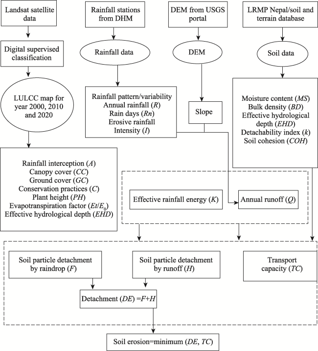
Table 1 Input parameter of RMMF model
Factor Parameter Definition and remarks
Rainfall R Annual or mean annual rainfall (mm)
Rn Number of rainy days per year.
I Typical value for intensity of erosive rain (mm h-1); 10 for temperate climates, 25 for tropical climates and 30 for strongly seasonal climates.
Soil MS Soil moisture content at field capacity or 1/3 bar tension (% w w-1).
BD Bulk density of the top soil layer (Mg m-3).
EHD Effective hydrological depth of soil (m); depend on vegetation/ crop cover, presence or absence of surface crust, presence of impermeable layer within 0.15 m of the surface.
K Soil detachability index (g J-1) defined as the weight of soil detached from the soil mass per unit of rainfall energy.
COH Cohesion of the surface soil (kPa)
Landform S Slope steepness (°).
Land Cover A Proportion between 0 and 1 of the rainfall intercepted by the vegetation or crop cover.
Et/E0 Ratio of actual (Et) to potential (E0) evapo-transpiration
C Crop cover management factor; combines the C and P factors of the Universal Soil Loss Equation.
CC Percentage canopy cover, expressed as a proportion between 0 and 1.
GC Percentage ground cover, expressed as a proportion between 0 and 1.
PH Plant height (m), representing the height from which raindrops fall from the crop or vegetation cover to the ground surface.
(4) Data processing
DEM derivatives, such as slope and aspect maps were generated from DEM. The data processing steps for database creation are illustrated in Fig. 4.
Fig. 4 Data processing steps for database creation
(5) Image classification and accuracy assessment
1) Image classification
For year 2000, 2010 and 2020 LULCC map from ICIMOD was used. For image classification procedure, Google Earth Engine (GEE) platform was used. Composite image consisting of image of all the seasons for the time frame was produced on GEE. Four land cover classes namely forest area, agriculture area, barren areas and water bodies were selected and training samples for each land cover class was selected. Maximum likelihood classifiers were selected for supervised classification. After classification, it was exported to TIFF format and was downloaded for further analysis.
2) Accuracy assessment
Assessing accuracy of digital image classification output is very important. Accuracy assessment is usually performed either using a new set of ground truth data or by comparing with a previously classified reference map for selected sampling points.
In this study, the accuracy assessment was done using ground truth data for 2023 using Google earth. The design of the sampling program is critical. In this study, stratified random sampling method was applied for the ground data collection. Spatially distributed sample points were selected for each class in LULCC classification scheme. Each of these points were checked in the field or with higher resolution images (Google earth), where locations were inaccessible. Every match between classified LULCC map and ground truth information was counted as 1 and for mismatch, it was result in 0. Overall accuracy is defined as the ratio between the total number of samples which are correctly classified, and the total number of samples considered for the accuracy assessment. User’s accuracy corresponds to error of commission. It refers to the measurement of how many of the samples of a particular class matched correctly (Congalton et al., 2001).
${{A}_{u}}=\frac{Sampl{{e}_{uc}}}{Sampl{{e}_{ut}}}$
where, Au is user’s accuracy; Sampleuc is total number of samples that are correctly classified in a given category; Sampleut is total number of samples in that category.
On the other hand, the producer’s accuracy corresponds to errors of omission. It is a measure of how much land in each LULCC category was classified correctly. It is calculated as:
${{A}_{p}}=\frac{Sampl{{e}_{pc}}}{Sampl{{e}_{pt}}}$
where, Ap is producer’s accuracy; Samplepc is total number of samples which are correctly classified for a given category; Samplept is total number of samples that are classified to that particular category.
The Kappa coefficient estimates the agreement between a modeled scenario and reality (Congalton, 1991). It determines if the results displayed in an error matrix are significantly better than random (Lillesand et al., 2015). For an error matrix with number of rows and column, kappa coefficient is computed as:
$K=n\times Sum\times {{X}_{ii}}-\frac{Sum(X_{i}^{+}\times X_{j}^{+})}{{{n}^{2}}\times Sum(X_{i}^{+}\times X_{j}^{+})}$
The result is poor if K<0.4; the result is good if 0.4≤K≤0.75; the result is excellent if K>0.75. Where, Sum is total number of observations included in the error matrix; Xii is diagonal total; Xi+ is marginal row total (row i); Xj+ is marginal column total (column j); n is number of observations (Julius and Wright, 2005).

2.3 Assessment of soil erosion

The methodology used for soil erosion risk assessment used Revised Morgan-Morgan and Finney (RMMF) model in a raster GIS environment for the quantification of soil loss utilizing several input parameters, such as DEM derived slope; soil map and soil characteristics; plant parameters; Rainfall characteristics data; and Land use/cover maps was derived by digital classification of satellite data. In this study, a cell size or pixel of 30 m was chosen.

2.3.1 Soil erosion modeling

Different models have been developed to assess soil erosion. Among them, the Revised Morgan Morgan and Finney Model (RMMF) with the aid of GIS are used in this study. The RMMF model simplified the erosion processes into detachment of soil particles from the soil mass by raindrop impact and the transport of those particles by runoff. The results obtained by the model are most sensitive to changes in annual rainfall and soil parameters when erosion is transport-limited and to changes in rainfall interception and annual rainfall when erosion is detachment-limited. The model input parameters for RMMF modeling are listed in Table 1.

2.3.2 Model input parameter

For running the RMMF model, soil data (detachability, moisture content at field capacity of the surface soil layer, bulk density, and effective hydrological depth), rainfall data (annual rainfall, rain intensity and number of rainy days per year), land cover data (Agriculture, Forest and Barren land) and topographic data (slope gradient) were required.

2.3.3 Land use and land cover information

Land use/Land cover maps generated using Landsat TM/ satellite data were reclassified and imported into ILWIS software for further analysis. The percentage of rainfall contributing to permanent interception (A), the ratio of actual to potential evaporate transpiration (Et/E0), the crop cover management factor (C), canopy cover (CC), ground cover (GC), plant height (PH) and Effective hydrological depth (EHD) was used as plant parameters and values derived using various literatures are presented in Table 2.
Table 2 Input parameter of vegetation
Land use/cover type A C Et CC GC PH (m) EHD (m)
Forest 0.430 0.70 0.90 0.70 0.30 18.00 0.180
Agriculture land 0.250 0.50 0.670 0.50 0.50 2.00 0.120
Barren Land 0.00 1.000 0.050 0.00 0.00 0.00 0.05

Note: Data source: Morgan et al., 1984; Shrestha, 1997; Morgan, 2001 and Regmi et al., 2014.

2.3.4 Digital Elevation Model and slope gradient map

Slope gradient map is an important parameter in the RMMF model (Morgan, 2001), especially in computing soil particle detachment and transport capacity of overland flow values. DEM was downloaded from USGS database at 30 m intervals by using ArcGIS 10.8 and was be imported in ILWIS 3.3 Academic.

2.3.5 Rainfall data

Daily rainfall data was collected for 20 years period (2000 to 2020) of four stations (Thankot, Markhu Gaaun, Chisapanigadhi and Daman) of the Kulekhani Watershed from Department of Hydrology and Meteorology (DHM) Kathmandu, Nepal (Table 3). The annual rainfall and number of rainy days per year data was correlated with elevation. The rainfall map and rainy day maps were then generated for the watershed through DEM by using following regression equations:
Rainfall = 0.5516× DEM + 625.64
Rainy Days = 0.0364× DEM + 51.323
Table 3 Annual rainfall and number of rainy days per year
Station Elevation
(m)
Annual rainfall
(mm)
Number of rainy
days per year
Chisapani Gadhi 1729 2024.60 125.95
Markhu Gaun 1535 1373.16 107.88
Thankot 1457 1733.05 119.36
Daman 2265 1711.48 126.19

Note: Source: Department of Hydrology and Meteorology, Kathmandu.

where DEM is elevation (m). For assessing soil erosion, rainfall intensity is a very important parameter in RMMF soil erosion model. The intensity of erosive rain was taken as 10 mm h-1, which was suggested by Morgan (2001) for temperate climate areas.

2.3.6 Soil data

Soil texture and soil maps are rasterized and geo-referenced to fit the base map, with a grid size of 30m and then imported in ILWIS for RMMF soil erosion modeling. The soil parameters used are soil moisture content at field capacity (MS), bulk density of the top soil in g cm-3 (BD), the soil detachability index K and cohesion of the surface soil (COH). The values of soil inputs for the different soil types of the watershed were assigned as suggested by Morgan (2001) according to soil texture classes as shown in Table 4.
Table 4 Soil input parameter
Soil type MS (%) BD (g cm-3) K (g J-1) COH (kPa)
Loam 0.20 1.3 0.8 3.0
Sandy loam 0.28 1.2 0.7 2.0
Silt loam 0.25 1.3 0.9 3.0

Note: Source: Summarized in Morgan et al., 1982 and Morgan, 2001.

2.3.7 Operative function of RMMF soil erosion model

(1) Rainfall energy estimation
The rainfall energy is the potential ability of rainfall for separating the soil particles from the soil surface. It generally represents the summation of the kinetic energy of the individual raindrops that strike the soil. This revised model takes into account of the way rainfall is partitioned during interception and the energy of the leaf drainage.
The effective rainfall (ER, mm) is defined as the amount of precipitation that is actually added and stored in the soil becoming available to the plant and it was estimated as:
ER=R×A
where R (mm) is the mean annual precipitation and A (%) is the rainfall interception coefficient (describes the precipitation amount retained from vegetation or crop cover, taking values between 0 and 1).
The ER is divided into two portions—one that reaches the soil surface unhindered as direct through fall (DT) and one that is intercepted by the plant canopy, reaching the surface as leaf drainage (LD). The division is determined by the percentage canopy cover (CC), expressed as a proportion between 0 and 1.
LD=ER×CC
DT=ER×LD
The kinetic energy (KE (DT), J m-2) of direct through fall was calculated as a function of rainfall intensity (I, mm h‒1). In the absence of field measurements, a typical value of I per climatic region is used (10 for temperate climates, 25 for tropical climates, 30 for climates with intense seasonal variations like Mediterranean type/monsoon) (Morgan, 2001).
KE(DT)=DT×(9.81+11.25lgI)
The kinetic energy of leaf drainage (KE(LD), J m-2) was calculated as a function of the plant canopy height (PH) using the Brandt (1990) formula.
KE(LD)=(15.8×PH0.5)-5.87
where PH (m) is the height from which raindrops fall from the crop/vegetation cover to the ground surface.
Overall, the total energy of the ER (KE, J m-2) was calculated by:
KE=KE(DT)+KE(LD)
(2) Estimation of runoff
The procedure for estimating the annual runoff (Q; mm) remains unchanged. It is based on the method proposed by Kirkby (1976) which assumes that runoff occurs when the daily rainfall exceeds the soil moisture storage capacity (Rc; mm) and that daily rainfall amounts approximate an exponential frequency distribution. The annual runoff was obtained from:
Q=R×e-Rc/R0
where, Q = Annual runoff (mm), R = Annual rainfall (mm), Rc = Soil moisture storage capacity.
Rc=1000×MS×BD×EHD×(Et/E0)
where, MS = Soil moisture content at field capacity (% w w-1), BD = Bulk density (Mg m-3), EHD = Effective hydrological depth of the soil (m), Et/E0 = Ratio of actual (Et) to potential (E0) evapo-transpiration.
R0=Mean rainfall per rain day (R/Rn)
where, R=Annual rainfall (mm), Rn=Number of rain days per year.
(3) Soil particle detachment by raindrop impact
In the revised MMF model, rainfall interception was allowed for the estimation of rainfall energy. It was removed from the equation used to describe soil particle detachment by raindrop impact (F; kg m-2) which then simplifies to:
F=K×KE×10-3
where, F=Raindrop impact (kg m-2), K=Erodibility of the soil (g J-1), KE=Kinetic energy of the effective rainfall (J m-2).
(4) Soil particle detachment by runoff
Soil particle detachment by runoff is estimated using following formula;
H=Z×Q1.5 ×Sinmap(1-GC) ×10-3
where, H = Soil particle detachment by runoff, Z = Resistance of the soil i.e., 1/ (0.5COH), Q = Annual runoff (mm), Sinmap = It was obtained from slope map of the study area by using formula i.e., SIN (DEGGRD) *Slope map, GC = Percentage ground cover.
(5) Transport capacity of runoff
It was calculated by using following formula;
TC=C×Q2×Sinmap×10-3
where, TC = Transport capacity of runoff (kg m-2), C = Crop cover management factor and Q = Annual Runoff (mm).
(6) Estimation of total annual detachment
Total annual detachment (DE; kg m-2) was calculated by summing soil particle detachment by raindrop (kg m-2) and soil particle detachment by runoff (kg m-2).
Total annual detachment=F+H
where, F = Soil particle detachment by raindrop (kg m-2) and H = Soil particle detachment by runoff (kg m-2).
(7) Estimation of total annual soil erosion
It was calculated by comparing annual detachment (DE) to annual transport capacity (TC). The lesser of the two values indicate annual soil erosion rate (Meyer and Wischmeier, 1969).
Annual erosion=minimum (DE, TC)

2.3.8 Soil erosion risk classes

Model estimated soil erosion values were grouped into six soil erosion risk classes based on range of soil loss values. The soil erosion risk class was categorized as very low (soil loss: <5 t ha-1 yr-1), low (soil loss: 5-10 t ha-1 yr-), moderate (soil loss: 10-15 t ha-1 yr-1), moderately high (soil loss: 15-25 t ha-1 yr-1), high (soil loss: 25-50 t ha-1 yr-1) and very high (soil loss: >50 t ha-1 yr-1). Finally, soil erosion risk zonation map was generated using operative functions of RMMF model and in ILWIS software environment. Soil erosion risk assessment was studied LULC wise over the whole watershed.

3 Results

3.1 Land use and land cover (LULC) classification

Land Use and Land cover classification of Kulekhani Watershed showed that the forest area increased from 60.72% in 2000 to 62.43% in 2010 and finally increase to 64.75% of the total area in 2020 (Table 5). The Water body was found continuously increasing with lower rate i.e., 1.07% in 2000 and 2010 and finally 1.08% in 2020. Barren land has been found increased from 0.21% in 2000 to 0.26% in 2010 and finally to 0.35% in 2020. On the other hand, the agriculture area was found decreasing within these periods having 38% in 2000, 36.24% in 2010 and finally 33.82% in 2020 (Fig. 5).
Table 5 LULC in 2000, 2010 and 2020
Class name 2000 2010 2020
Area (ha) % Area (ha) % Area (ha) %
Forest area 7560.45 60.72 7772.69 62.43 8063.01 64.75
Agriculture area 4732.02 38.00 4513.48 36.24 4211.55 33.82
Barren area 26.19 0.21 32.15 0.26 43.29 0.35
Water body 133.11 1.07 133.45 1.07 133.92 1.08
Total 12451.77 100 12451.77 100 12451.77 100
Fig. 5 LULC map of Kulekhani Watershed in 2000, 2010 and 2020

3.1.1 Accuracy assessment of the classification

Various types of error could be seen in the classified land cover maps from remotely sensed images. It is necessary to find out those errors to make the generated land cover maps more reliable, easily interpretable and acceptable by users. The accuracy of the classified image is a very crucial part in any image analysis. So, accuracy of the classified map has been assessed and compared with the reference data using a confusion matrix.
With respect to reference data, classified data of each land class were analyzed and executed in GEE with a set of algorithms. The overall accuracy for 2022 was 90.5% with Kappa coefficient 0.85. So, Kappa of 0.85 means there is 85% better agreement than by chance alone in 2020 (Table 6). The overall accuracy of the study was found to be 85 percent with kappa near to 1 which is within the acceptable level and thus it was considered as valid research.
Table 6 Accuracy assessment of the classification
Class Forest area Agriculture area Barren land Water body Row total User accuracy (%)
Forest area 66 6 3 0 75 88
Agriculture area 2 85 2 1 90 94
Barren land 1 2 20 2 25 80
Water body 0 0 0 10 10 100
Column total 69 93 25 13 200
Producer accuracy (%) 96 91 80 77 Overall accuracy=90.5%
Kappa coefficient = 0.85

3.1.2 LULC change pattern

3.1.2.1 LULC change pattern for the period of 2000-2010

The change analysis showed that the forest area and barren area were increased from 7560.45 ha and 26.19 ha to 7772.69 ha and 32.15 ha respectively. Similarly, water area was found to increase from 133.11 ha to 133.45 ha. On the other hand, the agriculture area was found to decrease from 4732.02 ha to 4513.48 ha during the time period 2000-2010 (Table 7).
Table 7 Change pattern for the period of 2000-2010
Class (2010) Area 2010 (ha) Class (2000) Area 2000 (ha) Change in class Change in area (ha)
Forest area 7772.69 Forest area 7560.45 Forest area - Forest area 212.24
Agriculture area 4513.48 Agriculture area 4732.02 Agriculture area - Agriculture area -218.54
Barren area 32.15 Barren area 26.19 Barren area - Barren area 5.96
Water body 133.45 Water body 133.11 Water body - Water body 0.34

3.1.2.2 LULC Change pattern for the period of 2010-2020

The change analysis showed that the forest area and barren area were increased from 7772.69 ha and 32.15 ha to 8063.01 ha and 43.29 ha respectively. Similarly, water area was found to increase from 133.45 ha to 133.92 ha. On the other hand, the agriculture area was found to decrease from 4513.48 ha to 4211.55 ha during the time period 2000-2010 (Table 8).
Table 8 Change pattern for the period of 2010-2020
Class (2020) Area 2020 (ha) Class (2010) Area 2010 (ha) Change in class Change in area (ha)
Forest area 8063.01 Forest area 7772.69 Forest area - Forest area 290.32
Agriculture area 4211.55 Agriculture area 4513.48 Agriculture area - Agriculture area -301.93
Barren area 43.29 Barren area 32.15 Barren area - Barren area 11.14
Water body 133.92 Water body 133.45 Water bodies - Water body 0.47

3.1.2.3 LULC Change pattern for the period of 2000-2020

The change analysis showed that the forest area and barren area were increased from 7560.45 ha and 26.19 ha to 8063.01 ha and 43.29 ha respectively (Table 9). Similarly, water area was found to increase from 133.11 ha to 133.95 ha. On the other hand, the agriculture area was found to decrease from 4732.02 ha to 4211.55 ha during the time period 2000-2020(Fig. 6).
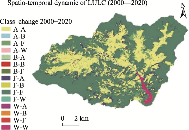
Table 9 Change pattern for the period of 2000-2020
Class (2020) Area 2020 (ha) Class (2000) Area 2000 (ha) Change in class Change in area (ha)
Forest area 8063.01 Forest area 7560.45 Forest area - Forest area 502.56
Agriculture area 4211.55 Agriculture area 4732.02 Agriculture area - Agriculture area 520.47
Barren area 43.29 Barren area 26.19 Barren area - Barren area 17.1
Water bodies 133.92 Water bodies 133.11 Water bodies - Water bodies 0.81
Fig. 6 Spatio-temporal dynamic of LULC (2000-2020)

Note: A: Agriculture area; B: Barren area; F: Forest area; W: Water body.

3.1.3 Soil erosion assessment

Revised Morgan-Morgan-Finney (RMMF) soil erosion model was used in ILWIS 3.3 and GIS (Geographic Information System) environment to calculate the soil loss and also to map soil erosion susceptibility in the watershed.

3.1.3.1 Digital Elevation Model

A Digital Elevation Model (DEM) represents the continuously varying topographic surface of the Earth, and it is a common data source for terrain analysis and other spatial applications (Moore et al., 1993). The DEM of the Kulekhani Watershed is shown in Fig. 7.
Fig. 7 Digital Elevation Model (DEM) of Kulekhani Watershed

3.1.3.2 Soil types of the watershed

The soil of the Kulekhani Watershed is mainly classified into three texture classes namely, Silty loam, Loam and Sandy loam (Table 10).
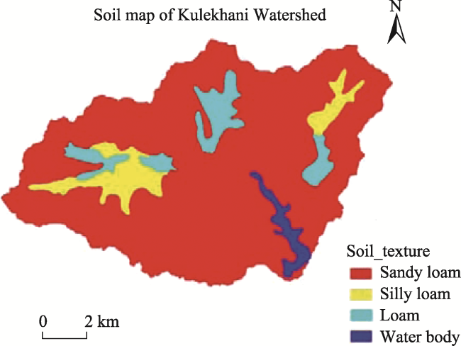
Table 10 Area of soil texture class
Soil texture class Total area (ha)
Sandy loam 10554.66
Silty loam 874.44
Loam 812.34
In the study area, the occurrence of sandy loam is high, silty loam has medium and loam has low proportion respectively. The texture class of the study area is presented in Table 10 and in Fig. 8.
Fig. 8 Soil map of the Watershed

3.1.3.3 Rainfall condition of the watershed

The average annual rainfall and average annual rainy days of the study area in four stations with elevations 1457-2265 m is collected from Department of Hydrology and Meteorology. In 2000, average annual rainfall was found to be high in station with elevation 1729 m which was 2157.36 mm (Table 11). Similarly, the average annual rainy days was found to be high i.e., 133.33 days which elevation 1729 m.
Table 11 Average annual rainfall and rainy days of 2000
S.N. Elevation (m) Rainfall (mm) Rainy days (days)
1 1729 2157.36 133.33
2 1535 1439.74 117.86
3 1457 1927.41 119.57
4 2265 1707.18 122
In 2010, average annual rainfall was found to be high in stations with elevation 1729 m which was 2078 mm (Table 12). Similarly, the average annual rainy days was found to be high i.e., 126.68 days which elevation 1729 m.
Table 12 Average annual rainfall and rainy days of 2010
S.N. Elevation (m) Rainfall (mm) Rainy days (day)
1 1729 2078.31 126.68
2 1535 1414.8 113.19
3 1457 1807.78 120.19
4 2265 1711.26 126.45
In 2020, average annual rainfall was found to be high in station with elevation 1729 m which was 2024.60 mm. On the other hand, the average annual rainy days was found to be high i.e., 126.18 days which elevation 2265 m (Table 13).
Table 13 Average annual rainfall and rainy days of 2020
S.N. Elevation (m) Rainfall (mm) Rainy days (days)
1 1729 2024.60 125.95
2 1535 1373.16 107.87
3 1457 1733.04 119.35
4 2265 1711.48 126.18

3.1.3.4 Soil Erosion in different LULC (2000-2020)

In this study, Revised Morgan, Morgan and Finney (RMMF) soil erosion model was used in GIS (Geographic Information System) environment to predict soil loss and to map soil erosion risk in the watershed. Various soil erosion factors such as LULC, soil, terrain- slope and rainfall were used in the model to assess current rate of soil loss and mapping of soil erosion risk areas. The modeling was done for the year 2000, 2010 and 2020. LULC wise range and weighted average annual soil losses in the watershed (Table 14).
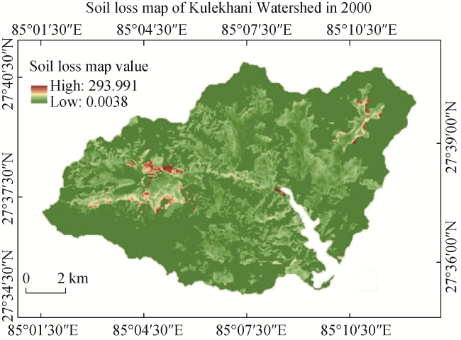
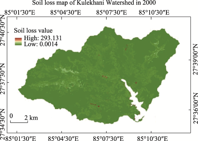
Table 14 LULC class wise average soil loss of the watershed
Year LULC class Minimum (t ha−1 yr−1 ) Maximum (t ha−1 yr−1 ) Average soil loss (t ha−1 yr−1 ) Weighted average soil loss
(t ha−1 yr−1 )
2000 Forest area 0.0038 0.2242 0.114 8.64
Agricultural area 0.4453 42.5339 21.4896
Barren area 6.4255 293.9912 150.20835
2010 Forest area 0.0024 0.2022 0.1023 7.12
Agriculture area 0.4422 35.9345 18.18835
Barren area 6.5522 293.4507 150.00145
2020 Forest area 0.0014 0.2242 0.1128 7.30
Agricultural area 0.4453 38.7258 19.58555
Barren area 6.7434 293.1306 149.937
Soil losses were comparatively lower under forest land and agriculture land and were maximum for barren land. In year 2000, soil loss under the forest land varied from 0.0038 to 0.2242 t ha−1 yr−1 and from 0.4453 to 42.5339 t ha−1 yr−1 in the agriculture land, and, in the barren land, it was about 6.4255 to 293.9912 t ha−1 yr−1 (Fig. 9).
Fig. 9 Soil loss map of the watershed in 2000 (t ha−1 yr−1)
Similarly, in year 2020, soil loss in the forest land varied from 0.0014 to 0.2242 t ha−1 yr−1 and from 0.4453 to 38.7258 t ha−1 yr−1 in the agriculture land and, in the barren land, it was about 6.7434 t ha−1 yr−1 to 293.1306 t ha−1 yr−1 (Fig. 10).
Fig. 10 Soil loss map of the watershed in 2020 (t ha−1 yr−1)

3.1.4 Erosion susceptibility assessment

Six soil susceptible classes were categorized based on potential soil loss values. The extent of soil erosion susceptible classes for the whole watershed is presented in Table 15. It indicates that the very low erosion susceptible class is in increasing trend from 2000 to 2020 from 7416.73 ha to 7874.75 ha. On the other hand, the very high soil erosion susceptible class is also decreasing from 2000 to 2020 from 143.4 ha to 122.9 ha.
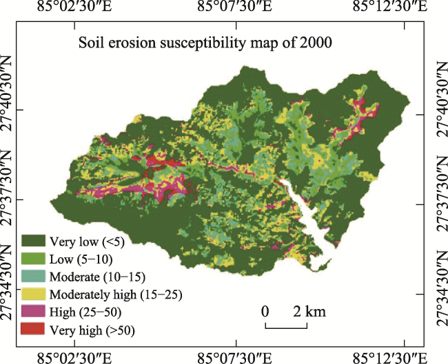
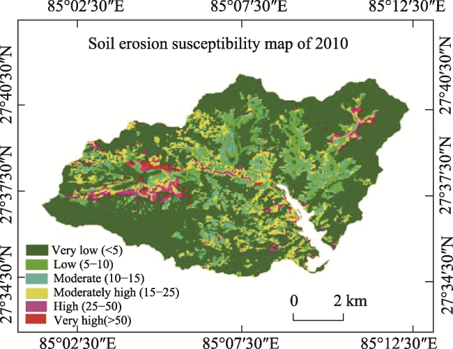
Table 15 Erosion susceptible classes of the Kulekhani Watershed in different time period
Erosion
susceptible class
Average soil loss range (t ha−1 yr−1) Area in 2000 (ha) Area in
2010 (ha)
Area in 2020 (ha)
Very low <5 7416.73 7766.41 7874.75
Low 5-10 577.49 572.83 556.34
Moderate 10-15 1146.58 1075.8 1137.91
Moderately high 15-25 1929.11 1729.08 1636.32
High 25-50 436.74 381.41 315.27
Very high >50 143.4 119.99 122.9
In 2000, very low soil erosion susceptible class was seen dominant in forest area whereas very high soil erosion susceptible class was dominant in the agriculture area and in vicinity to the barren areas (Fig. 11).
Fig. 11 Soil erosion susceptibility map of 2000 (t ha−1 yr−1)
In 2010, very low soil erosion susceptible class was seen dominant in forest area followed by agricultural area whereas very high soil erosion susceptible class showed the similar trend as of 2000 which was dominant in the agriculture area and in vicinity to the barren areas (Fig. 12).
Fig. 12 Soil erosion susceptibility map of 2010 (t ha−1 yr−1)
In 2020, very low soil erosion susceptible class was seen dominant in forest area followed by agricultural area since the agriculture area as found to be increased whereas very high soil erosion susceptible class showed the similar trend as of 2000 and 2010 which was dominant in the agriculture area and in vicinity to the barren areas (Fig. 13).
Fig. 13 Soil erosion susceptibility map of 2020 (t ha−1 yr−1)

4 Discussion

The RMMF model employs three key parameters for rainfall analysis: annual precipitation (R), the count of rainy days (Rd) per year, and rainfall intensity (I). For the value of I, a standard measurement of 10 mm h-1 was adopted, as recommended by Morgan (2001) for temperate climates. Research conducted by Bangladesh Unnayan Parishad (BUP) in 2007 and Shrestha et al. in 2000 demonstrates no substantial alteration in annual precipitation within Nepal. However, this current study indicates a decline in the average annual rainfall for Kulekhani. Notably, land use and land cover (LULC) changes have had a direct impact on soil loss. Analysis of LULC changes reveals a 0.14% increase in barren land between 2000 and 2020, significantly contributing to the heightened mean soil loss within the watershed area.
In contrast, the forested area expanded by 4.03% from 2000 to 2020, while the agricultural area experienced a decline of 4.18%. Table 6 illustrates the conversion of reduced agricultural land into forested and barren land. Additional studies highlight that soil erosion, a significant driver of soil degradation in Nepal’s middle mountain region, is primarily triggered and exacerbated by factors such as deforestation, overgrazing, intense agriculture, population pressure, over-cultivation, and rural development policies (Shrestha, 1997). Regarding the Kulekhani Watershed, this study reveals a decreasing trend in weighted average soil loss between 2000 and 2010, followed by a slight increase between 2010 and 2020. Notably, the highest soil loss occurred in 2000, with a weighted average of 8.64 t ha−1 yr−1. Barren land accounted for the maximum loss at 293.1306 t ha−1 yr−1, while the forest area experienced the least at 0.0038 t ha−1 yr−1. Similarly, in 2010, the weighted average soil loss was 7.12 t ha−1 yr−1, with barren land contributing the most at 293.4507 t ha−1 yr−1 and the forest area the least at 0.0024 t ha−1 yr−1. In 2020, the weighted average soil loss was 7.30 t ha−1 yr−1, with barren land accounting for the maximum loss at 293.1306 t ha−1 yr−1, and the forest area exhibiting the minimum at 0.0014 t ha−1 yr−1.
Shrestha (1997) reported higher annual soil loss rates, up to 56 t ha−1 yr−1, in rain-fed cultivation areas, while dense forests experienced lower soil losses of less than 1 t ha−1 yr−1. Soil loss in degraded forests ranged from 1 to 9 t ha−1 yr−1, and grazing lands had an estimated 8 t ha−1 yr−1. Sharma et al. (2011) observed a slight increase in the mean soil erosion potential of an agricultural watershed from 12.11 t ha−1 yr−1 in 1989 to 13.21 t ha−1 yr−1 in 2004. A study on the Adherikhola sub-basin in Western Nepal revealed that rainfed agriculture contributed to the highest soil loss at 32.5 t ha−1 yr−1, while forest cover and irrigated agricultural land experienced lower soil losses ranging from 0.01 to 0.4 t ha−1 yr−1 and 0.9 t ha−1 yr−1, respectively, resulting in an average estimated annual soil loss of 12.6 t ha−1 yr−1 (Dhakal, 2011).
In a similar vein, Upadhayay et al. (2018) assessed the relative impact of various land uses on suspended and streambed sediment loads in the Chitlang catchment. Utilizing a combination of the Bayesian mixing model, changes in land use patterns, and perception analysis, they identified major primary sediment sources as mixed and broadleaf forests during the pre-wet season, along with secondary sources like unpaved road tracks. However, the study lacked a comprehensive breakdown of contributions from different sources to anticipate variations in longer cycles.
The findings of this investigation were consistent with Uddin et al. (2018), who uncovered a decrease in the average soil erosion rate in Nepal from 8.76 t ha−1 yr−1 in 1990 to 7.9 t ha−1 yr−1 in 2010 due to shifts in land use and land cover. Their evaluation of land utilization and subsequent alterations also highlighted discrepancies in the distribution of soil erosion risk between 1990 and 2010. Nonetheless, the study failed to consider the diversity in rainfall patterns, soil conditions, and cultural practices, which contribute to the wide spectrum of erosion levels observed across different sites.
Likewise, the outcomes of this study echoed the results of Regmi et al. (2014), who calculated soil loss from various land uses in the Phewa watershed of Pokhara. Their estimations revealed an average annual soil loss of 0.2 t ha−1 yr−1 from dense forest, 0.5 t ha−1 yr−1 from medium to fairly dense forest, 1.1 t ha−1 yr−1 from open forest, 17.8 t ha−1 yr−1 from terraced agriculture, 0.3 t ha−1 yr−1 from valley agriculture, 3.7 t ha−1 yr−1 from bush/shrub land, 3.6 t ha−1 yr−1 from grassland, and a staggering 586.6 t ha−1 yr−1 from wasteland. Notably, wasteland exhibited the highest soil loss, while dense forest displayed the lowest, and a trend of increasing rainfall was also noted. The soil erosion susceptibility map depicted an augmentation in the zone of very low soil erosion susceptibility from 2000 to 2020, especially within forested regions. However, barren areas primarily exhibited these very low soil erosion susceptibility zones. In agricultural areas, soil erosion susceptibility diminished in low, moderate, and moderately high erosion zones. Mishra (2018) examined soil erosion risk using the RMMF model in Ritung Khola Sub-Watershed, Myagdi, Nepal. The study determined that 66.48% of the area posed very low and low soil erosion risk, 30.55% presented moderate and moderately high erosion risk, 2.86% exhibited high erosion risk, and 0.08% showcased very high erosion risk, aligning with the current study's findings. Another study conducted by Singh et al. (2023) evaluated the total annual soil loss in the Banas basin (encompassing an area of 6.82 million hectares) as 21.766 million tons. Maximum soil loss occurred in the extreme soil loss category (>50 t ha−1 yr−1) at 52 t ha−1 yr−1, while the minimum was in the low soil loss category (0-1 t ha−1 yr−1) at 0.8 t ha−1 yr−1. The present study's results also mirrored this trend.

5 Conclusions

This study has presented insights into the alterations in land cover over the previous two decades (2000, 2010, and 2020) and the resulting soil erosion within the categorized Land Use Land Cover (LULC) areas. The analysis of LULC classification for the Kulekhani Watershed demonstrated a progressive trend of forested area expansion, increasing from 60.72% in 2000 to 62.43% in 2010, and further to 64.75% in 2020. The aquatic body maintained its consistency at 1.07% between 2000 and 2010, with a marginal increment to 1.08% by 2020. Likewise, barren land witnessed an elevation from 0.21% to 0.26% between 2000 and 2010, and subsequently reaching 0.35% between 2010 and 2020. Conversely, agricultural land dwindled from 38% in 2000 to 36.24% in 2010, eventually declining to 33.82% by 2020. Notably, the analysis of LULC change indicated that, except for agricultural land use, all other land use categories exhibited growth from 2000 to 2020. The investigation revealed a diminishing trend in weighted average soil loss between 2000 and 2010, followed by a marginal increase from 2010 to 2020. The calculated soil loss stood at 8.64 t ha−1 yr−1 in 2000, 7.12 t ha−1 yr−1 in 2010, and 7.30 t ha−1 yr−1 in 2020. The gradual reduction in soil erosion during 2000-2010 primarily resulted from the expanded forested area. Conversely, the minor upturn in soil erosion between 2010 and 2020 could be attributed to indiscriminate road construction that overlooked proper soil and slope stabilization measures along roadways. Additionally, the erosion susceptibility map unveiled an escalating trend in the “very low risk” soil erosion zone from 2000 to 2020, particularly prominent within forested areas, followed by a transition from low to moderate susceptibility in agricultural regions. Barren areas exhibited a susceptibility ranging from moderately high to very high. This study unveiled a rise in soil loss within the watershed region, corroborated by field validation and interviews with key stakeholders. The escalation in reservoir sedimentation predominantly stems from haphazard rural road construction, contributing to frequent minor landslides along roadsides.
[1]
Abdulkareem J H, Pradhan B, Sulaiman W N A, et al. 2019. Prediction of spatial soil loss impacted by long-term land-use/land-cover change in a tropical watershed. Geoscience Frontiers, 10(2): 389-403.

DOI

[2]
Aksoy A Dowell D C, Snyder C. 2009. A multicase comparative assessment of the ensemble Kalman filter for assimilation of radar observations. Part I: Storm-scale analyses. Monthly Weather Review, 137(6): 1805-1824.

DOI

[3]
Atreya K, Sharma S, Bajracharya R M, et al. 2006. Applications of reduced tillage in hills of central Nepal. Soil and Tillage Research, 88(1): 16-29.

DOI

[4]
Bajracharya R M, Sherchan D P. 2009. Fertility status and dynamics of soils in the Nepal Himalaya:A review and analysis. In: Lucero D P, Boggs J E eds. Soil fertility. New York, USA: Nova Science Publishers Inc.: 111-135.

[5]
Bastola S, Seong Y J, Lee S H, et al. 2019. Assessment of soil erosion loss by using RUSLE and GIS in the Bagmati Basin of Nepal. Journal of the Korean GEO-environmental Society, 20(3): 5-14.

[6]
BUP (Bangladesh Unnayan Parishad). 2007. Enhancement of National Capacities in the Application of Simulation Models for the Assessment of Climate Change and its Impacts on Water Resources.

[7]
Chalise D, Kumar L, Spalevic V, et al. 2019. Estimation of sediment yield and maximum outflow using the IntErO model in the Sarada River Basin of Nepal. Water, 11(5): 952. DOI: 10.3390/w11050952.

[8]
Congalton R G. 1991. A review of assessing the accuracy of classifications of remotely sensed data. Remote Sensing of Environment, 37(1): 35-46.

DOI

[9]
Congalton R G. 2001. Accuracy assessment and validation of remotely sensed and other spatial information. International Journal of Wildland fire, 10(4): 321-328.

DOI

[10]
Dhakal M. 2011. Climate change impacts on reservoir based hydropower generation in Nepal: A case study of Kulekhani Hydropower Plant. Diss., Pokhara, Nepal: Pokhara University.

[11]
DSCWM (Department of Soil Conservation and Watershed Management). 2015. Soil Conservation and Watershed Management Programs.

[12]
Efthimiou N. 2019. Development and testing of the Revised Morgan-Morgan-Finney (RMMF) soil erosion model under different pedological datasets. Hydrological Sciences Journal, 64(9): 1095-1116.

DOI

[13]
FAO (Food and Agriculture Organisation of the United Nations). 2015. Status of the World’s Soil Resources (SWSR). Main Report. Rome, Italy: FAO.

[14]
Garcia-Ruiz J M, Begueria S, Lana-Renault N, et al. 2017. Ongoing and emerging questions in water erosion studies. Land Degradation & Development, 28(1): 5-21.

DOI

[15]
Julius S, Wright C C. 2005. The Kappa statistic in reliability studies: Use, interpretation, and sample size requirements. Physical Therapy, 85(3): 257-268.

PMID

[16]
Kirkby M J. 1976. Tests of the random network model, and its application to basin hydrology. Earth Surface Processes, 1(3): 197-212.

DOI

[17]
Li L, Wang Y, Liu C. 2014. Effects of land use changes on soil erosion in a fast developing area. International Journal of Environmental Science and Technology, 11(6): 1549-1562.

DOI

[18]
Li Z, Liu W Z, Zhang X C, et al. 2011. Assessing the site-specific impacts of climate change on hydrology, soil erosion and crop yields in the Loess Plateau of China. Climate Change, 105(1-2): 223-242.

DOI

[19]
Lillesand T, Kiefer R W, Chipman J. 2015. Remote sensing and image interpretation. Hoboken, USA: John Wiley and Sons, Inc.

[20]
LRMP. 1986. Land Resources Mapping Project. Kathmandu, Nepal: Kenting Earth Science.

[21]
Meyer L D, Wischmeier W H. 1969. Mathematical simulation of the process of soil erosion by water. Transactions of the ASAE, 12(6): 754-758.

DOI

[22]
Mishra S K. 2018. Soil erosion assessment by using Revised Morgan, Morgan Finney (RMMF) Model in GIS framework: A case study of Ritung Khola Sub-Watershed. Myagdi District, Nepal.

[23]
Moore I D, Gessler P E, Nielsen G A E, et al. 1993. Soil attribute prediction using terrain analysis. Soil Science Society of America Journal, 57(2): 443-452.

DOI

[24]
Morgan R P, Finney H J, Morgan D D. 1982. Stability of agricultural ecosystems: Documentation of a simple model for soil erosion assessment. Laxenburg, Austria: International Institute for Applied Systems Analysis.

[25]
Morgan R P C. 2001. A simple approach to soil loss prediction: A revised Morgan, Morgan Finney Model. Catena, 44(4): 305-322.

DOI

[26]
Morgan R P C, Morgan D D V, Finney H J. 1984. A predictive model for the assessment of erosion risk. Journal of Agricultural Engineering Research, 30: 245-253.

DOI

[27]
Nippon Koei Co. Ltd. 1983. Kulekhani Hydroelectric Project: Project Completion Report.

[28]
Persichillo M G, Bordoni M, Meisina C. 2017. The role of land use changes in the distribution of shallow landslides. Science of the Total Environment, 574: 924-937.

DOI

[29]
Pokharel B, Thapa P B. 2018. Assessment of rock slope stability in Kulekhani Watershed, central Nepal. Bulletin of Nepal Geological Society, 35: 179-183.

[30]
Pradhan B, Chaudhari A, Adinarayana J, et al. 2012. Soil erosion assessment and its correlation with landslide events using remote sensing data and GIS: A case study at Penang Island, Malaysia. Environmental Monitoring and Assessment, 184: 715-727.

DOI PMID

[31]
Regmi R R, Saha S K, Balla M K. 2014. Geospatial analysis of land use land cover change modeling at Phewa Lake Watershed of Nepal by using Cellular Automata Markov Model. International Journal of Current Engineering and Technology, 4(1): 260-267.

[32]
Sangroula D P. 2005. Sedimentation and sustainability of the Kulekhani Reservoir: A Himalayan case. Diss., Trondheim, Norway: Norwegian University of Science & Technology.

[33]
Sangroula D.P. 2005. Sedimentation and Sustainability of the Kulekhani Reservoir: A Himalayan Case; Norwegian University of Science & Technology: Trondheim, Norway, p. 283.

[34]
Schreier H, Brown S, Shah, P B. 1995. Challenges in mountain resource management in Nepal: Processes, trends and dynamics in middle mountain watersheds. In: Proceedings of a workshop held in Kathmandu, Nepal, 10-12 April, 1995. DOI: 10.53055/icimod.189.

[35]
Schwilch G, Adhikari A, Jaboyedoff M, et al. 2017. Impacts of outmigration on land management in a Nepali mountain area: Identifying emerging issues in disaster risk reduction, migration, climate change and sustainable development: Shaping debates and policies: 177-194. DOI: 10.1007/978-3-319-33880-4_11.

[36]
Sharma A, Tiwari K N, Bhadoria P B S. 2011. Effect of land use land cover change on soil erosion potential in an agricultural watershed. Environmental Monitoring and Assessment, 173: 789-801.

DOI PMID

[37]
Shrestha A B, Wake C P, Dibb J E, et al. 2000. Precipitation fluctuations in the Nepal Himalaya and its vicinity and relationship with some large scale climatological parameters. International Journal of Climatology: A Journal of the Royal Meteorological Society, 20(3): 317-327.

DOI

[38]
Shrestha S, Khatiwada M, Babel M S, et al. 2014. Impact of climate change on river flow and hydropower production in Kulekhani hydropower project of Nepal. Environmental Processes, 1: 231-250.

DOI

[39]
Shrestha D, Zinck J, Van E. 2004. Modelling land degradation in the Nepalese Himalaya. Catena, 57(2): 135-156.

DOI

[40]
Shrestha D P. 1997. Assessment of soil erosion in the Nepalese Himalaya: A case study in Likhu Khola Valley, Middle Mountain Region. Land Husbandry, 2(1): 59-80.

[41]
Singh M C, Sur K, Al-Ansari N, et al. 2023. GIS integrated RUSLE model-based soil loss estimation and watershed prioritization for land and water conservation aspects. Frontiers in Environmental Science, 11: 1136243. DOI: 10.3389/fenvs.2023.1136243.

[42]
Subedi L, Acharya K K. 2016. Tracing the Mahabharat Thrust (MT) on the basis of lithology and microstructures around Bhainse-Manahari area, central Nepal. Journal of Nepal Geological Society, 51: 39-48.

DOI

[43]
Tiwari K R, Sitaula B K, Bajracharya R M, et al. 2009. Runoff and soil loss responses to rainfall, land use, terracing and management practices in the Middle Mountains of Nepal. Acta Agriculturae Scandinavica Section B—Soil and Plant Science, 59(3): 197-207.

[44]
Uddin K, Abdul Matin M, Maharjan S. 2018. Assessment of land cover change and its impact on changes in soil erosion risk in Nepal. Sustainability, 10(12): 4715. DOI: 10.3390/su10124715.

[45]
Upadhayay R, Smith H G, Griepentrog M, et al. 2018. Community managed forests dominate the catchment sediment cascade in the mid-hills of Nepal: A compound-specific stable isotope analysis. Science of the Total Environment, 637: 306-317.

Outlines

/