
Journal of Resources and Ecology >
Can the Yangtze River Delta Urban Agglomeration Policy Promote Green High-quality Development? Evidence from the Digital Economy and Green Total Factor Productivity
Received date: 2023-05-21
Accepted date: 2023-08-20
Online published: 2023-12-27
Supported by
The National Natural Science Foundation of China(71873003)
The Key Program of the Department of Education of Anhui Province(SK2020A0131)
The Research Project on Humanities and Social Sciences for Higher Education of Anhui Province(YJS20210256)
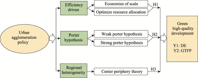
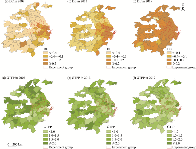
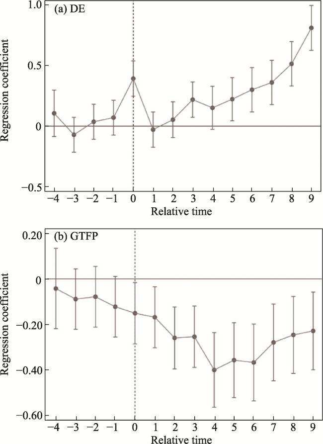
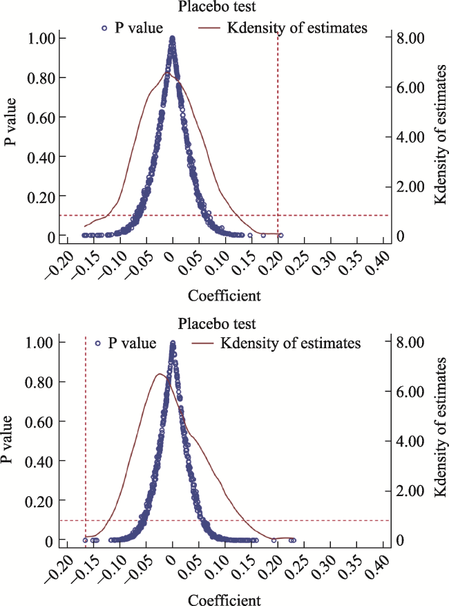
Urban agglomerations should meet the dual requirements of economic growth and green development, and there is currently an urgent need to improve the efficiency of green development. Therefore, we analyzed the impact of the Yangtze River Delta Urban Agglomeration (YRDUA) policy on the digital economy (DE) and green total factor productivity (GTFP) using the time-varying difference in difference model (DID). The marginal contribution of this study is an evaluation of the long-term effect of the YRDUA policy on green high-quality development. Based on the perspective of the “Porter Hypothesis”, this study examined the similarities and differences in the impacts of urban agglomeration on DE and GTFP. The results show that the policy promotes the urban DE index, but significantly inhibits urban GTFP. This means that the overall impact of urban agglomeration policy on green high-quality development in the Yangtze River Delta (YRD) is still in the “weak Porter Hypothesis” state, the technological innovation and efficiency improvement stimulated by urban agglomeration policies are not enough to significantly improve GTFP, and the “strong Porter Hypothesis” is not tenable. In addition, the heterogeneity analysis shows that the policy has a more obvious role in promoting the green high-quality development of central cities, large and medium-sized cities and innovative cities. The level of urban public service supply shows a threshold effect. When it develops to a certain scale, the urban agglomeration policy has significant positive impacts on both DE and GTFP.
JIN Cai , HUI Baohang , LI Tan . Can the Yangtze River Delta Urban Agglomeration Policy Promote Green High-quality Development? Evidence from the Digital Economy and Green Total Factor Productivity[J]. Journal of Resources and Ecology, 2024 , 15(1) : 105 -116 . DOI: 10.5814/j.issn.1674-764x.2024.01.009
Table 1 Input and output indicators and descriptions |
| First indices | Second indices | Description |
|---|---|---|
| Input | Labor | Employees of the unit (104 persons) |
| Capital | Capital stock of fixed assets (104 yuan) | |
| Energy | Electricity consumption in the society (104 kWh) | |
| Expected output | Economic output | Regional GDP (104 yuan) |
| Unexpected output | Environmental contamination | Industrial wastewater (104 t) |
| Industrial SO2 (t) | ||
| Industrial soot (t) |
Table 2 Variables and descriptive statistics |
| Variable | Description | Number | Mean | SD | Min | Max |
|---|---|---|---|---|---|---|
| DE | Digital economy | 1287 | -0.17 | 0.64 | -0.98 | 8.81 |
| GTFP | Green total factor productivity | 1287 | 1.43 | 0.36 | 0.29 | 5.73 |
| DID | Policy dummy variable | 1287 | 0.16 | 0.37 | 0.00 | 1.00 |
| ln pgdp | Logarithm of per regional GDP | 1287 | 10.58 | 0.65 | 8.68 | 12.20 |
| ln inter | The logarithmic number of Internet broadband households | 1287 | 13.18 | 0.96 | 10.54 | 17.76 |
| ln fin | Loan balance as a percentage of GDP | 1287 | 17.18 | 1.07 | 14.52 | 21.40 |
| ln fdi | Logarithm of actually used foreign capital | 1287 | 10.62 | 1.26 | 7.07 | 14.46 |
| Ind | Proportion of the added value of the secondary industry in the regional GDP | 1287 | 0.50 | 0.09 | 0.15 | 0.77 |
Table 3 The results of the models |
| Variable | DE | GTFP | ||
|---|---|---|---|---|
| (1) | (2) | (3) | (4) | |
| DID | 0.143** (0.058) | 0.200*** (0.048) | -0.108** (0.045) | -0.165*** (0.035) |
| ln pgdp | 0.482*** (0.096) | 0.192** (0.095) | ||
| ln inter | 0.539** (0.269) | -0.139** (0.065) | ||
| ln fin | -0.393** (0.168) | 0.158 (0.116) | ||
| ln fdi | -0.045** (0.021) | 0.057** (0.025) | ||
| Ind | -1.056** (0.335) | -0.682* (0.345) | ||
| Constant | -0.539*** (0.023) | -4.453** (1.995) | 1.280*** (0.018) | 7.170*** (2.195) |
| Time FE | √ | √ | √ | √ |
| Individual FE | √ | √ | √ | √ |
| R2 | 0.344 | 0.619 | 0.054 | 0.010 |
| N | 1287 | 1287 | 1287 | 1287 |
Note: * P<0.1, ** P<0.05, *** P<0.01; Robust standard errors are shown in parentheses. |
Table 4 Heterogeneity of the center-periphery cities |
| Variable | Central cities | Peripheral cities | ||
|---|---|---|---|---|
| DE | GTFP | DE | GTFP | |
| DID | 0.423* (0.217) | -0.072 (0.179) | 0.001 (0.044) | -0.003 (0.065) |
| Control variables | Yes | Yes | Yes | Yes |
| Constant | 0.341*** (0.081) | 9.453*** (6.741) | -4.385* (2.308) | 9.980*** (3.276) |
| Time FE | √ | √ | √ | √ |
| Individual FE | √ | √ | √ | √ |
| R2 | 0.229 | 0.013 | 0.839 | 0.054 |
Note: * P<0.1, ** P<0.05, *** P<0.01. Robust standard errors are shown in parentheses. |
Table 5 Heterogeneity of city population scales |
| Variable | Small cities (≤3 million) | Medium-sized cities (3-6 million) | Large cities (>6 million) | |||
|---|---|---|---|---|---|---|
| DE | GTFP | DE | GTFP | DE | GTFP | |
| DID | 0.092 (0.055) | -0.311** (0.089) | 0.170*** (0.046) | -0.106* (0.059) | 0.378* (0.202) | -0.112** (0.050) |
| Control variables | √ | √ | √ | √ | √ | √ |
| Constant | -4.472*** (1.397) | -4.331 (7.566) | -3.140** (1.529) | 6.547*** (2.109) | 5.241 (6.895) | 13.185*** 0.0155 |
| Time FE | √ | √ | √ | √ | √ | √ |
| Individual FE | √ | √ | √ | √ | √ | √ |
| R2 | 0.792 | 0.040 | 0.793 | 0.017 | 0.001 | 0.016 |
Note: * P < 0.1, ** P < 0.05, *** P < 0.01. Robust standard errors are shown in parentheses. “≤ 3 million”, “3-6 million” and “> 6 million” refer to the resident population of less than 3 million, 3 million to 6 million and more than 6 million respectively. |
Table 6 Heterogeneity of innovative city |
| Variable | Innovative cities | Non-innovative cities | ||
|---|---|---|---|---|
| DE | GTFP | DE | GTFP | |
| DID | 0.213*** | -0.171*** | 0.118*** | -0.132** |
| (0.102) | (0.042) | (0.041) | (0.058) | |
| Control variables | √ | √ | √ | √ |
| Constant | 0.227 | 9.641*** | -3.473** | 6.279** |
| (5.808) | (3.387) | (1.304) | (2.480) | |
| Time FE | √ | √ | √ | √ |
| Individual FE | √ | √ | √ | √ |
| R2 | 0.192 | 0.008 | 0.796 | 0.011 |
Note: * P < 0.1, ** P < 0.05, *** P < 0.01. Robust standard errors are shown in parentheses. |
Table 7 Threshold regression results |
| Variable | DE | GTFP |
|---|---|---|
| DID (U≤U1) | 0.066** (0.032) | -0.005 (0.031) |
| DID | 6.175*** | 0.829*** |
| (U1<U≤U2) | (0.256) | (0.111) |
| DID | -1.385*** | -0.222** |
| (U>U2) | (0.135) | (0.110) |
| Constant | -3.114*** (0.363) | 1.430*** (0.008) |
| Time FE | √ | √ |
| Individual FE | √ | √ |
| R2 | 0.538 | 0.028 |
Note: * P < 0.1, ** P < 0.05, *** P < 0.01. Robust standard errors are shown in parentheses. |
| [1] |
|
| [2] |
|
| [3] |
|
| [4] |
|
| [5] |
|
| [6] |
|
| [7] |
|
| [8] |
|
| [9] |
|
| [10] |
|
| [11] |
|
| [12] |
|
| [13] |
|
| [14] |
|
| [15] |
|
| [16] |
|
| [17] |
|
| [18] |
|
| [19] |
|
| [20] |
|
| [21] |
|
| [22] |
|
| [23] |
|
| [24] |
|
| [25] |
|
| [26] |
|
| [27] |
|
| [28] |
|
| [29] |
|
| [30] |
|
| [31] |
|
| [32] |
|
| [33] |
|
| [34] |
|
| [35] |
|
| [36] |
|
| [37] |
|
| [38] |
|
| [39] |
|
| [40] |
|
| [41] |
|
| [42] |
|
| [43] |
|
| [44] |
|
| [45] |
|
| [46] |
|
| [47] |
|
| [48] |
|
| [49] |
|
| [50] |
|
| [51] |
|
| [52] |
|
/
| 〈 |
|
〉 |