
Journal of Resources and Ecology >
A Spatial Convergence Analysis of China’s Urban Eco-efficiency: Perspectives based on Local Government Competition
Received date: 2023-02-04
Accepted date: 2023-06-15
Online published: 2023-11-10
Supported by
The Natural Science Foundation of Hunan Province(2023JJ40104)
The Research Foundation of Hunan Provincial Social Science Achievement Review Committee(XSP22YBZ091)
The Research Foundation of Education Bureau of Hunan Province(23B0887)
The National Social Science Foundation of China(17BJL119)
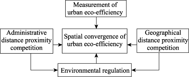
Regional collaborative governance of the ecological environment is an important way to promote the sustainable development of urbanization, and local government competition is a characteristic institutional factor that is often ignored in the process of regional ecological environmental governance in China. This study selected the panel data of 278 prefecture-level cities from 2006 to 2018 in China, and used the spatial convergence regression model and the mediation effect model to analyze the spatial convergence of urban eco-efficiency (UEE) and its mechanism from the perspective of local government competition. The results show several empirical patterns. First, the UEE follows a tendency of convergence that narrows the regional gap of urban eco-efficiency, and spatial interaction factors are the keys affecting the convergence of UEE. Second, local government competition, as a characteristic institutional factor, plays an important role in promoting the spatial convergence of UEE, and the effect of administrative distance proximity competition is stronger than that of geographical distance proximity competition. The UEE increases by 0.114 percentage points when its degree of competitive pressure increases by 1 percentage point. Third, the competitive pressure leads to strict environmental regulation policies, which generally improve UEE and thus narrow its gap with advanced cities. Finally, local government competition has heterogeneous effects on urban eco-efficiency. Specifically, under the pressure of local government competition, the environmental regulations improve the UEE in the east and key environmental protection cities, while the central and non-key environmental protection cities experience the opposite effect. The results of this study suggest that if UEE is further introduced into the administrative performance evaluation index systems of local officials, the regional gap of environmental and economic development could be narrowed through ecological competition.
CHEN Peirong , YIN Xiangfei , LU Mingxuan . A Spatial Convergence Analysis of China’s Urban Eco-efficiency: Perspectives based on Local Government Competition[J]. Journal of Resources and Ecology, 2024 , 15(1) : 90 -104 . DOI: 10.5814/j.issn.1674-764x.2024.01.008
Table 1 Input-output variables and data description |
| Category | Variable | Data and description |
|---|---|---|
| Inputs | Capital (K) | The “perpetual inventory method” was used to estimate the capital stock. The calculation formula is: ${{K}_{it}}={{I}_{it}}+(1-{{\delta }_{t}}){{K}_{it-1}}$, in which ${{I}_{it}}$ is the fixed asset investment of the city i in year t. The capital stock in the initial year was obtained by the method of Young (2003), and the depreciation rate ${{\delta }_{t}}$ was derived from Shan (2008) |
| Labor (L) | Employed population at the end of the year | |
| Land resources (B) | Urban construction land area (Bai et al., 2018) | |
| Water resources (W) | Total urban water supply minus domestic water consumption to obtain water resources input | |
| Energy (E) | The electricity consumption data automatically recorded by the meter is more accurate, and there is a high correlation between electricity consumption and energy consumption (Li et al., 2013). Referring to Li and Xu (2018), this paper used prefecture-level city power consumption data as proxy variables | |
| Desired output | GDP (U) | Real GDP was considered as the most important desirable output |
| Undesired outputs | Waste water (D) | Industrial waste water emission |
| Waste gas (S) | Industrial sulfur dioxide emission |
Note: Due to the inconsistent statistical caliber of industrial (smoke) dust in the sample period, this variable was not used as an unexpected output. To eliminate the influences of price factors, all economic data were adjusted to the corresponding prices in 2006. |
Table 2 Regression results for the convergence of urban eco-efficiency |
| Variable | (1) Model Ⅰ | (2) Model Ⅱ | (3) Model Ⅲ | (4) Model Ⅳ |
|---|---|---|---|---|
| Lag(ln UEE) | -0.135*** | -0.283*** | -0.413*** | -0.438*** |
| (-5.94) | (-7.97) | (-37.19) | (-35.41) | |
| IND | 0.018* | 0.024*** | 0.051*** | |
| (1.67) | (3.29) | (7.13) | ||
| TEC | 0.004*** | 0.004*** | 0.004*** | |
| (5.90) | (19.19) | (18.69) | ||
| FDI | 3.39* | 1.001 | 1.369* | |
| (1.85) | (1.22) | (1.93) | ||
| PERGDP | 0.013*** | 0.027*** | 0.027*** | |
| (4.47) | (26.40) | (26.47) | ||
| $\eta \text{ }$ | 0.103*** | 0.051* | ||
| (3.83) | (1.76) | |||
| $\rho $ | 0.173*** | 0.122*** | ||
| (6.36) | (3.68) | |||
| City effect | Yes | Yes | Yes | Yes |
| Time effect | - | - | No | Yes |
| Hansen test | 0.875 | 0.343 | ||
| AR(2) | 0.343 | 0.478 | ||
| R2 | 0.679 | 0.571 | ||
| F/LogL | 8.12 | 11.10 | 1275.10 | 1072.32 |
| Obs. | 3614 | 3614 | 3614 | 3614 |
| Convergence rate | 0.1450 | 0.3327 | 0.5327 | 0.5763 |
Note: The t-statistics for the coefficients are in parentheses; ***, **, and * indicate 1%, 5%, and 10% significance levels, respectively; and the same notation is used in subsequent tables. |
Table 3 Benchmark estimated results |
| Variable | Sys-GMM | Two-way FE | ||
|---|---|---|---|---|
| (1) | (2) | (3) | (4) | |
| LGC1 | 0.114*** (3.55) | 0.219*** (18.66) | ||
| LGC2 | 0.102** (2.19) | 0.167*** (3.69) | ||
| Lag(ln UEE) | 0.598*** (7.78) | 0.445*** (4.86) | ||
| Control variable | Yes | Yes | Yes | Yes |
| R2 | 0.198 | 0.168 | ||
| F | 21.380 | 32.373 | 46.813 | 101.81 |
| Hansen test | 0.308 | 0.204 | ||
| AR(2) | 0.881 | 0.867 | ||
| Obs. | 3614 | 3614 | 3614 | 3614 |
Table 4 Estimated results of the mediation effect |
| Variable | (1) ln UEE | (2) ER | (3) ln UEE |
|---|---|---|---|
| LGC | 0.114*** (3.55) | 0.002** (1.99) | 0.106*** (3.65) |
| ER | 0.505** (2.20) | ||
| Lag(ER) | 0.769*** | ||
| (31.67) | |||
| Lag(ln UEE) | 0.598*** (7.78) | 0.643*** (9.48) | |
| Control variable | Yes | Yes | Yes |
| Hansen test | 0.308 | 0.131 | 0.896 |
| AR(2) | 0.881 | 0.278 | 0.773 |
| F | 21.380 | 580.320 | 22.603 |
| Obs. | 3614 | 3614 | 3614 |
Table 5 Heterogeneity analysis of different regions |
| Variable | ER | ln UEE | ||||||
|---|---|---|---|---|---|---|---|---|
| (1) East | (2) Central | (3) West | (4) North-east | (5) East | (6) Central | (7) West | (8) North-east | |
| LGC | 0.005*** | 0.004** | 0.006* | 0.002 | 0.103*** | 0.137*** | 0.236*** | 0.156*** |
| (6.91) | (2.08) | (1.76) | (1.42) | (3.40) | (3.31) | (2.76) | (2.12) | |
| ER | 0.755** | -2.056*** | 1.483* | 2.211** | ||||
| (1.98) | (-4.30) | (1.68) | (2.41) | |||||
| Lag(ER) | 0.658*** | 0.737*** | 0.748*** | 0.881*** | ||||
| (132.11) | (25.38) | (31.47) | (16.83) | |||||
| Lag(ln UEE) | 0.553*** | 0.275*** | 0.473*** | 0.227*** | ||||
| (7.03) | (9.53) | (4.40) | (9.79) | |||||
| Control variable | Yes | Yes | Yes | Yes | Yes | Yes | Yes | Yes |
| Hansen test | 0.232 | 0.477 | 0.666 | 0.827 | 0.864 | 0.114 | 0.999 | 0.230 |
| AR(2) | 0.235 | 0.329 | 0.050 | 0.424 | 0.368 | 0.466 | 0.739 | 0.207 |
| F | 318.121 | 288.750 | 166.120 | 117.269 | 12.611 | 37.542 | 12.314 | 24.917 |
| Obs. | 1313 | 1157 | 702 | 442 | 1313 | 1157 | 702 | 442 |
Table 6 Heterogeneity analysis in the key and non-key environmental protection cities |
| Variable | Key environmental protection cities | Non-key environmental protection cities | ||||
|---|---|---|---|---|---|---|
| (1) ln UEE | (2) ER | (3) ln UEE | (4) ln UEE | (5) ER | (6) ln UEE | |
| LGC | 0.130** | 0.004*** | 0.055** | 0.085** | 0.000 | 0.058* |
| (2.60) | (11.74) | (2.11) | (2.39) | (0.85) | (1.68) | |
| ER | 2.387*** | 0.158 | ||||
| (3.06) | (1.01) | |||||
| Lag(ln UEE) | 0.555*** | 0.529*** | 0.491*** | 0.475*** | ||
| (7.61) | (8.32) | (6.90) | (8.12) | |||
| Lag(ER) | 0.340*** | 0.538*** | ||||
| (31.90) | (19.10) | |||||
| Control variable | Yes | Yes | Yes | Yes | Yes | Yes |
| Hansen test | 0.235 | 0.144 | 0.693 | 0.136 | 0.177 | 0.111 |
| AR(2) | 0.894 | 0.508 | 0.932 | 0.899 | 0.253 | 0.875 |
| F | 15.107 | 142.392 | 13.310 | 25.156 | 456.452 | 19.707 |
| Obs. | 1417 | 1417 | 1417 | 2197 | 2197 | 2197 |
Table 7 Heterogeneity analysis in different periods |
| Variable | 2006-2012 | 2013-2018 | ||||
|---|---|---|---|---|---|---|
| (1) ln UEE | (2) ER | (3) ln UEE | (4) ln UEE | (5) ER | (6) ln UEE | |
| LGC | 0.120*** | 0.006** | 0.114*** | 0.189** | 0.003*** | 0.127*** |
| (3.72) | (2.34) | (3.65) | (2.44) | (3.18) | (3.85) | |
| ER | -0.546*** | 1.808*** | ||||
| (-3.48) | (4.25) | |||||
| Lag(ln UEE) | 0.420*** | 0.162*** | 0.363*** | 0.509*** | ||
| (8.18) | (9.65) | (7.22) | (8.62) | |||
| Lag(ER) | 0.679*** | 0.834*** | ||||
| (16.18) | (27.15) | |||||
| Control variable | Yes | Yes | Yes | Yes | Yes | Yes |
| Hansen test | 0.149 | 0.051 | 0.122 | 0.095 | 0.301 | 0.210 |
| AR(2) | 0.901 | 0.261 | 0.754 | 0.756 | 0.861 | 0.348 |
| F | 17.740 | 99.250 | 51.955 | 64.619 | 124.920 | 19.134 |
| Obs. | 1946 | 1946 | 1946 | 1668 | 1668 | 1668 |
Table 8 Estimated results of the robustness analysis |
| Variable | (1) ln UEE | (2) ER | (3) ln UEE |
|---|---|---|---|
| LGC | 0.127** | 0.003** | 0.069** |
| (2.11) | (2.24) | (2.25) | |
| ER | 0.760** | ||
| (2.18) | |||
| Lag(ln UEE) | 0.512*** | 0.493*** | |
| (5.56) | (7.57) | ||
| Lag(ER) | 0.731*** | ||
| (25.04) | |||
| Control variable | Yes | Yes | Yes |
| Hansen test | 0.101 | 0.116 | 0.630 |
| AR(2) | 0.256 | 0.272 | 0.242 |
| F | 22.978 | 264.394 | 14.517 |
| Obs. | 3614 | 3614 | 3614 |
| [1] |
|
| [2] |
|
| [3] |
|
| [4] |
|
| [5] |
|
| [6] |
|
| [7] |
|
| [8] |
|
| [9] |
|
| [10] |
|
| [11] |
|
| [12] |
|
| [13] |
|
| [14] |
|
| [15] |
|
| [16] |
|
| [17] |
|
| [18] |
|
| [19] |
|
| [20] |
|
| [21] |
National Bureau of Statistics (NBS). 2022. Significant progress has been made in promoting energy conservation and consumption reduction:14 in the series of reports on achievements in economic and social development since the 18th CPC National Congress. https://www.gov.cn/xinwen/2022-10/08/content5716734.htm.
|
| [22] |
|
| [23] |
|
| [24] |
|
| [25] |
|
| [26] |
|
| [27] |
|
| [28] |
|
| [29] |
|
| [30] |
|
| [31] |
|
| [32] |
|
| [33] |
|
| [34] |
|
| [35] |
|
| [36] |
|
| [37] |
|
| [38] |
|
| [39] |
World Business Council for Sustainable Development (WBCSD), 1996. Eco-efficient leadership for improved economic and environmental performance. Conches-Geneva, Switzerland.
|
| [40] |
|
| [41] |
|
| [42] |
|
| [43] |
|
| [44] |
|
| [45] |
|
| [46] |
|
| [47] |
|
| [48] |
|
| [49] |
|
| [50] |
|
| [51] |
|
| [52] |
|
/
| 〈 |
|
〉 |