Resources and Economy

How Does Spatial Heterogeneity Affect Industrial Outputs? Literature Review and Research Prospects

  • XIE Ailiang , 1, 2, * ,
  • Fauziah CHE LEH 1 ,
  • Norimah RAMBELI 3
Expand
  • 1. Department of Geography and Environment, Faculty of Human Sciences, Education University of Sultan Idris, Tanjong Malim, Perak 35900, Malaysia
  • 2. Department of History and Culture, Linyi University, Linyi, Shandong 276005, China
  • 3. Department of Economics, Faculty of Management and Economics, Education University of Sultan Idris, Tanjong Malim, Perak 35900, Malaysia
* XIE Ailiang, E-mail:

Received date: 2022-07-20

  Accepted date: 2023-01-10

  Online published: 2023-10-23

Supported by

The Philosophy and Social Science Foundation of China(21BGL150)

Abstract

The impact of spatial heterogeneity on industrial outputs is a new important topic in economic geography. A considerable amount of research literature has accumulated, but the academic community lacks a systematic and comprehensive review and consensus on this topic. This study carried out research by mining the relevant classical literature. This investigation first combed the connotation of spatial heterogeneity, which is both corresponding to and related to spatial dependence. Theorists generally acknowledge that there is spatial heterogeneity in the process of industrial outputs. Then this study summarizes the logical basis, relationship coordination, measurement and other aspects of the effect of spatial heterogeneity on industrial outputs. In analyzing the impact of spatial heterogeneity on industrial outputs, we should not ignore the spatial dimension, but must also pay attention to the heterogeneity of individual enterprises. Industrial output analysis needs to be based on the relationship between spatial heterogeneity and spatial dependence. The influence of spatial heterogeneity on industrial outputs and the degree of differences among observation objects can be measured by econometric methods. The common indicators for measuring and quantitatively describing the impact of spatial heterogeneity on industrial outputs mainly include semivariogram, the spatial expansion model and the geographical weighted regression model. Finally, some directions of future research are pointed out in order to provide useful ideas for future theoretical research and industrial practice.

Cite this article

XIE Ailiang , Fauziah CHE LEH , Norimah RAMBELI . How Does Spatial Heterogeneity Affect Industrial Outputs? Literature Review and Research Prospects[J]. Journal of Resources and Ecology, 2023 , 14(6) : 1217 -1226 . DOI: 10.5814/j.issn.1674-764x.2023.06.010

1 Introduction

Industrial outputs have always been a major topic of research and discussion in economic geography (Fujita and Krugman, 2004). Industrial outputs refer to the sum of the value of goods and services produced by the resident units in various departments of the national economy in a certain period of time, so it reflects the total results of the production and business activities of various departments of the national economy (Leontief, 1936). Industrial outputs are the product of the comprehensive influence of many factors. Among them, the congenital conditions and core elements that determine regional industrial competitiveness and industrial outputs are location factors (Herliana, 2015). The first law of geography indicates that everything is related to everything else, but near things are more closely related than distant things (Tobler, 1970). Geographical things or attributes are related to each other in spatial distribution. However, with the increase in geographical distance, this correlation decreases. As a result, geographical things or attributes are unbalanced in their spatial distributions, and become more complex. This kind of spatial heterogeneity and its complexity are generally called spatial heterogeneity. For a certain region, any economic phenomenon within its scope has a certain correlation with the economic phenomena of adjacent regions, showing a certain spatial autocorrelation and spatial imbalance (Anselin, 1989). The spatial correlation between regions is a phenomenon that cannot be ignored in the study of regional economic problems (Liu, 2020). Therefore, Goodchild (2004a, 2004b) proposed the second law of geography. The law of spatial heterogeneity (Law of spatial heterogeneity) leads to differences between ground objects, that is, heterogeneity. Spatial heterogeneity is divided into spatial local heterogeneity and spatial stratified heterogeneity.
When the growth of the spatial dimension is not given enough attention, it may lead to biased results and even lead to wrong conclusions. In order to emphasize this problem, economic geographers require that spatial dependence and spatial heterogeneity be taken into account when examining regional industrial outputs (Anselin et al., 2000; Mameli et al., 2012; Murshed et al., 2020; Billé, 2021; Yan et al., 2022). Spatial heterogeneity is an important feature of the spatial performance of industrial outputs (Liu et al., 2021), and mainly refers to the uneven spatial distribution and complexity of various economic factors that affect industrial outputs (Alvarado, 2021). The spatial heterogeneity of these economic factors leads to the different degrees of attractiveness of different regions to different economic actors (Anselin, 2001a), which makes the industrial outputs of various regions show great differences in space, and there are also obvious differences among enterprises (Scott, 1988). To put spatial heterogeneity simply, if we think that enterprises are heterogeneous and always interact with each other, then the different regions in which they exist will also be heterogeneous and interact. Tran and Santarelli (2017) used a unique panel dataset of 60 two-digit industries across 64 provinces from 2000 to 2010 in Vietnam to investigate the importance of spatial and sectoral heterogeneity in an analysis of the determinants of entrepreneurship and to empirically explore the interaction effect of geographic conditions and industry dynamism. Yu et al. (2021) developed a new spatial heterogeneity model in the form of a mixed geographically weighted panel regression with the spatial Durbin model (MGWPR-SDM). Using this model, this study adds to the debate over the possible existence of a Swedish paradox in China.
Previous studies have shown that there is structural instability in both spatial dependence and spatial heterogeneity in regional industrial outputs (Dall’Erba et al., 2008). At the same time, the industrial outputs of a specific region have a strong spatial spillover effect on adjacent regions (Du et al., 2022). The differences in geographical environments play an important role in the industrial layout (Breschi and Malerba, 1997). Isard (1951) pointed out that the research on the balance of regional industrial outputs mainly comes from two different theoretical explanations or predictions. First, per capita income tends to a steady level “β Convergence”. Second, due to the existence of externalities, knowledge spillovers, specialization and other factors, the gap in economic growth is widening. Although many studies have empirically tested the above two trends, most of them adopted a common assumption of parameter homogeneity. Therefore, they proposed to relax the homogeneity assumption of policy variables and set the heterogeneity parameters based on the development level of a country or region in order to reflect the spatial differences of variables affecting industrial outputs, such as the spatial heterogeneity of policy variables (Ramajo, 2008). Through the component regression method (Lu et al., 2014), this study tests whether the impacts of physical capital investment, human capital investment, population growth and regional location differences on industrial outputs will show different growth distributions due to the different locations of a city.
Against the background of increasingly fine social division among industries, spatial heterogeneity has an increasingly profound impact on industrial outputs. The impact of spatial heterogeneity on industrial outputs has become an important research hotspot in the field of economic geography. Therefore, it is of great theoretical significance to systematically analyze and sort out the existing research results on how spatial heterogeneity affects industrial outputs in order to clarify its theoretical context. Previous studies have generated a great deal of valuable research results on spatial heterogeneity in the field of industrial outputs, and the research purposes, perspectives and methods also show diversity. However, the reality is that heterogeneous space is a normal state that cannot be ignored. What is spatial heterogeneity? How does spatial heterogeneity affect industrial outputs? How can the impact of spatial heterogeneity on industrial outputs be measured? These research propositions have quietly become the focus of theoretical circles.

2 Literature retrieval and research approaches

In the first stage, terms related to spatial heterogeneity and industrial outputs were used to search in the “arbitrary field” of the Scopus database, and 4808 publications were obtained. Among them, a total of 4754 items were published after 2002. The retrieval date was July 2, 2022. The retrieved items were all read, analyzed and sorted, and the cited references were screened to avoid omitting relevant studies as much as possible. This process finally yielded 65 core studies. In the second stage, the theoretical basis and variables for measuring the impact of spatial heterogeneity on industrial outputs were first traced and classified. Then the logical basis was sorted and an analysis framework was built. The third stage involved reflecting on and criticizing the research on the impact of spatial heterogeneity on industrial outputs, and the variable definitions, measurement ideas and research prospects were put forward. The literature search results showed that the research on the impact of spatial heterogeneity on industrial outputs began to attract academic attention around 2002 (i.e., the number of published studies exceeded 10 for the first time in 2002), and the number of studies increased rapidly after 2012 (i.e., the number of published literatures exceeded 100 for the first time in 2012), which indicates a research field with great potential (Fig. 1).
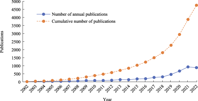
Fig. 1 Trend of publications amount on the impact of spatial heterogeneity on industrial outputs from 2002 to 2022

3 Interpreting the connotation of spatial heterogeneity

The discussion of spatial heterogeneity first appeared in Anselin’s (1989) understanding of the essence of spatial heterogeneity. Anselin wrote that spatial heterogeneity (spatial difference) refers to the characteristics of things and phenomena in each spatial location that are different from those in other locations. The specific empirical model shows that variables, parameters and error terms change with changes in the investigated location (space). His research has provided a basic theoretical framework for subsequent researchers, and served also as the theoretical guidance for later scholars in this field.
Based on the proposition that spatial econometrics is different from traditional econometrics, LeSage (1999) proposed the dual characteristics of spatial econometrics, namely spatial dependence and spatial heterogeneity. Qualitatively speaking, spatial heterogeneity refers to the change in spatial relations, or the existence of differentiated relations at specific points in space (Allen, 1999). At the same time, this qualitative characteristic of spatial heterogeneity can also be quantified. Li and Reynolds (1995) defined spatial heterogeneity as the spatial complexity and variability of systems or system attributes. Complexity involves the qualitative or type description of system attributes (Fusco et al., 2018), while variable heterogeneity should consider the quantitative description of system attributes (Kotliar and Wiens, 1990). Structural heterogeneity and functional heterogeneity are two major components of spatial heterogeneity (De Marsily et al., 2005). Brunsdon et al. (1999) considered the factor of spatial heterogeneity in their study of regional economy and economic geography. When the geographical space lacks homogeneity, there are unbalanced geographical structures such as developed and underdeveloped areas, core and marginal areas. Heterogeneity can also be manifested as the spatial instability of economic behavior or economic relations (Hess, 2004). Spatial heterogeneity is also a common unstable relationship of economic behavior between economic units in space in the process of economic activities (Ramajo, 2008), and this unstable relationship can be identified by spatial statistics and measurement methods (Anselin, 2019). Specifically, in the economic model, both the variance of the investigation variables and the error term of the model parameters change with changes in location (Anselin, 2001a).

4 The logical basis of spatial heterogeneity affecting industrial outputs

4.1 The logical basis of spatial heterogeneity affecting industrial output needs to be developed based on spatial dimension

Considering the characteristics of social development and economic growth that occur independently at different times and places on the earth, as well as the obvious regional differences and the great inequality in the welfare of people between various regions of the world, a comprehensive economic theory or social theory should include the two dimensions of time and space (Isard, 1956). Therefore, when analyzing the impact of spatial heterogeneity on industrial outputs, we cannot ignore the spatial dimension. Although there is no consensual explanation for the scientific definition of space in theoretical circles (Sack, 1974; Montello and Sutton, 2006; Wither, 2009; Liu et al., 2017; Olechnicka et al., 2019; Komilova et al., 2021), the recognition of the existence of “space” and “spatial attributes” is surprisingly consistent, and gives “space” various natural, social and economic attributes (Haining, 2003). Bourdieu (1998) believed that space itself does not have practical significance, and it is important only when human economic and social activities give it a corresponding position. Lefebvre (2012) examined the important role of space from the perspectives of history, society and space, and put forward the concept of “the production of space”. Space is both the means of production and the object of consumption, and has the characteristics of scarcity (Lash et al., 1993). As the means of production, space is the carrier of wealth and material sources (Corsín, 2003). As the object of consumption, space is consumed in production (Mansvelt, 2008). These views are particularly important for strengthening the spatial dimension thinking in the research on spatial heterogeneity affecting industrial outputs. Postmodernism continues and develops Lefebvre’s view in its criticism of “static space”, “physical space”, “relational space” and “perceptual space”, and believes that space is neither neutral nor simple geometric figures, but is constantly produced through social spatial relations (Murphet, 2004; Portugali, 2006; Lagopoulos, 2011; Kemppainen, 2022). Space is the product of the integration of cultural, social, political and economic relations (Kozhevnikov, 2020). Industrial outputs come from space, which are affected by space and feed back to industrial outputs (Hausmann et al., 2014). Ultimately, the decision of spatial significance still comes down to people's social and economic practice.

4.2 The logical basis of spatial heterogeneity affecting industrial output needs to fully consider the heterogeneity of individual enterprises

Neoclassical economics takes “rational economic man” and “perfect competition” as the starting point and logical framework of its economic analysis (Colander, 2000). However, when faced with complex social, political and economic activities, neoclassical economics often lacks explanatory power, which determines the limitations and relativity of the scope of application of neoclassical economics (Kjosavik, 2003). Numerous so-called “abnormal situations” in the real economy are difficult to resolve in terms of realistic explanations and predictions within the theoretical framework of neoclassical economics (Berg and Gigerenzer, 2010). Therefore, behavioral economists put forward the concept of heterogeneous economic actors and revised the assumption of homogeneous economic actors (Axtell, 2007). The so-called heterogeneous economic actors are individuals with behavioral heterogeneity, such as choice and judgment determined by the endogenous preferences of economic individuals (Thaler, 2016). Similarly, there is heterogeneity among individual enterprises in the process of industrial outputs. In analyzing the impact of spatial heterogeneity on industrial outputs, considering the heterogeneity of individual enterprises is inevitable.
Starting from the heterogeneity of individual enterprises, space, as an individual with an independent attribute, has also received attention. When exploring the characteristics of space from the socio-economic attributes of space, it is easy to see that space is a collection of specific natural, economic and social endowments (Simone et al., 2021). The diversity and complexity of these spatial elements constitute the diversity and complexity of space. Specifically, the supply and demand levels of different spaces are very different, the carrying capacities of regions are also different, and there are great differences in the intensity and density of economic activities in each space (Ciccone and Hall, 1996). The profit seeking nature of individual enterprises will achieve higher efficiency through “capitalization of Decentralized Economy” and the “uneven geographical distribution of resources” (Bocken et al., 2014). The problem of preference seems to be attributed to psychological tendencies. Whether space is regarded as an independent phenomenon or as an event attribute of spatial analysis, “space” can be distinguished and separated, and its spatial utility can be evaluated. Ignoring the existence of individual heterogeneity will greatly affect the ability of theory to explain reality, which will then reduce the predictive analysis ability of the model.

5 Industrial output analysis needs to be carried out based on spatial characteristics

Revealing the relationships between things is the core of scientific research (Portugali, 2006). Generally speaking, spatial effects can be divided into spatial dependence and spatial heterogeneity (Basile, 2014). If spatial heterogeneity is a manifestation of unstable relations, spatial dependence can be defined as the consistency between economic behavior units and locations (Anselin, 2001b).
When doing quantitative research on regional industrial outputs, we often need to rely on geographical sampling measurement data (Nordhaus, 2006). When the sampling data of industrial outputs have regional factors, spatial heterogeneity and spatial dependence must be considered (Bai, 2019). In other words, the industrial output data and information collected from spatial points may not be independent of each other, but there is often a positive or negative spatial correlation, which means that the samples in a place and the samples in adjacent areas show similar or opposite trends. This condition is spatial dependence. In the process of exploring the spatial dependence of industrial outputs, although a certain region may have a spatial correlation with several adjacent regions, this correlation may not be constant. Perhaps there is a strong positive correlation between this region and the specific relationship being investigated in some adjacent regions, while there is also a positive correlation between the same relationships investigated in other adjacent regions, but this positive correlation is relatively weak. This is an example of spatial heterogeneity.
The spatial heterogeneity and spatial dependence of industrial outputs together constitute a spatial effect. From the perspective of spatial econometrics, these two characteristics are also the most critical characteristics that distinguish Spatial Econometrics from general econometrics. Both spatial heterogeneity and spatial dependence cause the sampling data of industrial outputs to have regional characteristics. With changes in the spatial sampling data, the previously established variable relationship also needs to change.
At the same time, it should be noted that spatial heterogeneity and spatial dependence often exist in the spatial data of industrial outputs at the same time, and the two go hand in hand. Therefore, the test of one property in the model usually affects the test of another property. Spatial heterogeneity has also become a huge challenge because it is difficult to separate from spatial dependence.
Research on the impact of spatial heterogeneity on industrial output is constantly developing. Understanding the research progress of disciplines related to the impact of spatial heterogeneity on industrial output will help to clarify and further explain the basic concepts and core contents of the spatial heterogeneity effects on industrial output. As an important research perspective for geographers, spatial cognition can build a good research framework for assessing the impact of spatial heterogeneity on industrial output. The main logic of research on the impact of spatial heterogeneity on industrial output in the field of economic geography can be summarized as the continuous deepening of the understanding of spatial heterogeneity and the continuous exploration of how to apply industrial output realistically. For this reason, such research attempts to build a theoretical framework from causality to cognitive process, and then to structure, rule and behavioral decision-making (Fig. 2).
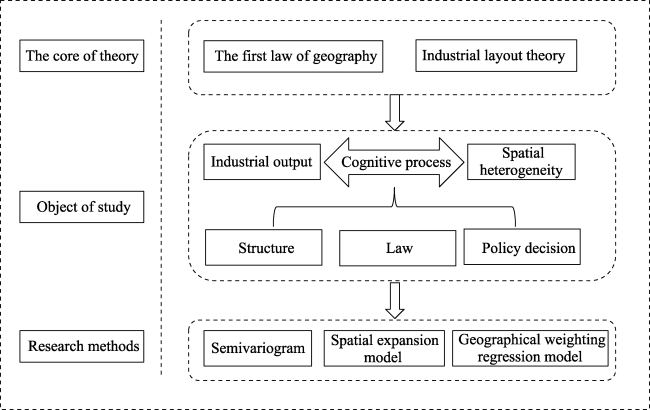
Fig. 2 Theoretical framework for analyzing the impact of spatial heterogeneity on industrial output
The concept and connotation of spatial heterogeneity affecting industrial output are constantly developing. Initially, they represent the subjective cognitive image of static industrial output spatial information. Then they express the process of spatial perception and spatially-aware information processing on how industrial output is affected by spatial heterogeneity, as well as the judgment of participating in their own behavioral decision-making. The spatial heterogeneity influences the industrial output, which is characterized by a combination of dynamic subjective processing and static image result representation.
The influence of spatial heterogeneity on industrial output should pay further attention to the relationship between cognitive subject attributes and cognitive processes, the scale effect of cognitive objects, and the impact of non-representational factors on the spatial cognitive results. Admittedly, research on the impact of spatial heterogeneity on industrial output includes not only the subject and object, process, structure and their interrelationships, but also the perspective of higher dimensions and more related objects in the future in order to reflect the complexity of subjective cognition.

6 Quantitative description of the impact of spatial heterogeneity on industrial outputs

When analyzing the impact of spatial heterogeneity on industrial outputs, we can often obtain useful information from the deconstruction and reconstruction of the spatial structure of industrial outputs (Brenner, 1999). From the perspective of metrology, spatial heteroscedasticity, spatial coefficient of variation, random coefficients and the change of the spatial structure can be regarded as the metrological reflection of spatial heterogeneity. In the existing research, three kinds of indicators are used most often.

6.1 Semivariogram

The semivariogram is one of the key functions in geostatistics for studying spatial heterogeneity. It is a continuous function used to describe the continuous spatial variation of geographical factors, reflecting the changes between observations at different distances. There is a functional relationship between the semivariogram of data points and the distances between data points (Lin and Chen, 2004). The nugget and range of the semivariogram model may give some direction to understanding the spatial distribution at the unobserved scale, such as the subdistrict level. The semivariogram model also provides better information than other measures of spatial autocorrelation, i.e., the Moran coefficient. The semivariogram model’s parameters give information about variance (sill), inter-dependency in terms of geographical distance (range) and the nugget effect, which reveals interesting information about the latent inter-relationship of the characteristics within a particular area (Pardo-Iguzquiza and Chica-Olmo, 2008). Basile (2014) presented a semiparametric framework which allows us to relax the linearity assumption and, simultaneously, model spatial dependence and unobserved heterogeneity. In general, SVM types yield prediction accuracy that is better than other types of regression, and GPR types produce better DEM accuracy based on experiments (Setiyoko et al., 2019). For example, Srikhum and Simon (2010) used a non-stationary semivariogram to analyze real estate transaction data, and confirmed a degree of spatial autocorrelation (positive or very positive autocorrelation) between neighboring properties. Fleming (2000) discussed spatial statistics and econometrics for models in fisheries economics.
In the process of analyzing the impact of spatial heterogeneity on industrial output, the semivariogram is usually used to measure the spatial autocorrelation of field types of spatial data. The implementation of the method takes the size of the statistical correlation coefficient as a function of distance, and measures its correlation through the differences of distances and attributes. Semivariogram modeling is similar to fitting the least squares in regression analysis. The goal of the semivariogram is to minimize the deviation between the point and other points according to some criteria, in order to calculate the parameters of the curve. In order to accurately describe the impact of spatial heterogeneity on industrial production, the weighted quadratic programming method, genetic algorithm and pattern search method can be used to optimize the semivariogram. At the same time, the influence of weights on the fitting accuracy of a semivariogram needs to be considered.

6.2 Spatial expansion model

The spatial expansion model was first proposed by Casetti (1972). Based on an “initial model”, this model is extended to a “terminal model” by changing the parameters of some variables. When an “initial model” cannot meet some of the requirements or has some deficiencies, the more appropriate approach is not to abandon it, but to reconstruct it or expand on its basis. In the case of spatial dependence, following theoretical arguments from new economic geography, and endogenous growth models, this phenomenon has been associated with the existence of externalities that cross regional borders (Aguilar, 1999). For example, Burnett (2012) used a computable general equilibrium model with integrated commercial and residential land data to estimate the impact of urban growth, both in sector origin and growth mechanism, on urban spatial expansion as measured by density (population, employment, and commercial), residential lot size, and urban land conversion. Kang and Ma (2021) developed a theoretical framework that explored the formation mechanism and expansion process of urban agglomerations from the perspective of industrial evolution, and identified the development issues and their causes by taking the Yangtze Delta and Beijing-Tianjin-Hebei urban agglomerations as case studies.
In the process of actual industrial outputs, the selected object will inevitably be affected by the natural, economic and social environment. Uncertainties, external disturbances and input-output constraints occur from time to time. In this case, the industrial outputs under the effect of spatial heterogeneity can be regarded as a discrete system with uncertainty and unknown interferences. The output error is extended to the spatial expansion model, which forms a new extended state space model with less conservatism. The system control law that is designed based on this model can adjust the dynamic response of the system state and the output tracking error respectively, while eliminating the steady-state error.
The statistical data of industrial output are typical time-space data. In a time section, it is spatial data and has spatial and geographical relevance. However, in a specific geographical location, the observations are a time series, with the correlation of time factors. Especially when the industrial output analysis needs to consider the industrial structure, it is more suitable to use the spatial expansion model. The spatial expansion model is a function that expands the parameters in the model into spatial structure, in which the spatial structure can be reflected by distance, direction, spatial coordinates, location, and other attributes. On the other hand, compared with geographical weighting, the spatial expansion model is more helpful for model testing assumptions. In many cases, the spatial extension model can effectively describe the spatial continuity of data.

6.3 Geographical weighting regression model

Geographically weighted regression (GWR) was first used in spatial econometric analysis by Brunsdon et al. (1996). It has subsequently been widely used in recent years as a modeling technology that can simply and effectively deal with spatial nonstationarity. The GWR Model is a regression estimation method with spatial variable coefficients, which is an extension of the general linear regression model (Fotheringham and Charlton, 1998). It extends the traditional regression framework, allowing local rather than global parameter estimation (Yu et al., 2020). By assuming that the regression coefficient is the location function of the geographical location of the observation point in the linear regression model, the spatial characteristics of the data are incorporated into the model, so that the influences of the explanatory variables on the explained variables may be different in different regions, thereby showing spatial complexity, autocorrelation and variability. The GWR model creates conditions for analyzing the spatial characteristics of regression relationships, and can effectively solve the problem of spatial instability (Brunsdon et al., 1998).
Huang and Leung (2002) used the GWR technique to study regional industrialization in Jiangsu province, and found significant differences between the ordinary linear regression (OLR) and GWR models. The relationships between the level of regional industrialization and various factors show considerable spatial variability. Considering the spatial differences among the provinces in China, the GWR model has been used to investigate the impacts of industrial structure, energy intensity, urbanization and environmental regulation on carbon transfer (Wang et al., 2021). Thissen et al. (2016) applied a neo-classical regional growth model using GWR and showed that the degree of competition in trade and services between sectors moderates regional structural growth.
Considering the characteristics of industrial outputs, it is necessary to build an endogenous spatiotemporal weight matrix that is suitable for panel data spatial metrology local analysis based on the holographic mapping of nearest neighbor local points to the target analysis local points. On this basis, and based on the decomposition of local point parameter estimation and the analysis of the overall properties of the model, the panel spatio-temporal geographical weighted regression model method is systematically constructed. The panel spatiotemporal GWR model based on holographic mapping comprehensively analyzes the direct and indirect paths of influencing effects between local points in space. Both the peer effect of the nearest local point in space and the endogenous dynamics of the local point in space are considered. At the same time, based on the optimal spatial bandwidth and optimal time bandwidth, the effective nearest local points are included, which makes the analysis of the regularity and heterogeneity of the spatial dependence of local points more accurate.
Compared with general linear regression models, GWR models can embed the spatial attributes of industrial output data, deal with the non-stationary spatial relationships of control variables, and effectively reflect the spatial non-stationary characteristics of regression coefficients. GWR models can analyze the spatial characteristics of industrial output. Based on a geographic weighted regression model, multi-scale geographic weighted regression can relax the parameter scale constraints of different explanatory variables, allow different explanatory variables of the regression model to participate in the regression on different scales, and include the scale heterogeneity characteristics among variables in the regression equation. The GWR model takes into account the spatial characteristics of the factors affecting industrial output and the differences in regression parameters between regions. It reflects the spatial heterogeneity of data and reveals the spatial laws of the influencing factors. A geographically weighted regression model is not only easy to understand and operate, but can also show the estimation results of the model through clear analytic expressions, and the parameter estimation can also be statistically tested.

7 Conclusions

The above observations and research on the impact of spatial heterogeneity on industrial outputs show that there are at least three aspects of consensus in the theoretical community on the understanding of the impact of spatial heterogeneity on industrial outputs. One is the recognition that there is spatial heterogeneity in the process of industrial outputs. At the same time, this objective existence can have different forms of expression. It may be the differences of phenomena or things in the industrial space, the differences of the structure and function of the industrial space itself, or both. The concept of “spatial heterogeneity” conveys the idea that when spatial factors are introduced into industrial output analysis, the spatial characteristics, or the key characteristics of one space that are different from another, need to receive sufficient attention. Second, spatial heterogeneity is both corresponding to and related to spatial dependence. Investigating the impact of spatial heterogeneity on industrial outputs is usually carried out together with the investigation of spatial dependence. When studying the spatial elements of industrial outputs, we should not only observe the interactions and relationships between the elements, but also identify the strength of the role of different economic spaces. Third, the influence of spatial heterogeneity on industrial outputs and the degree of differences of the observation objects can be measured by econometric methods. Spatial measurement tools and means have been widely used in the field of industrial output research. In short, the existence of spatial heterogeneity means that in addition to exploring the overall industrial outputs, it is also necessary to identify local differences in industrial spatial patterns and reveal the characteristics of industrial spatial differences.
Due to the complexity of spatial heterogeneity affecting industrial outputs, the relevant theoretical interpretations and analyses show different scenarios, and the research on the impact of spatial heterogeneity on industrial outputs needs to be further expanded. There are still many theoretical gaps to be filled, and the relevant empirical research is relatively immature. Efforts should be made to more accurately measure the impact of spatial heterogeneity on industrial outputs; to use the research results of other disciplines on the impact of spatial heterogeneity on industrial outputs for economic research; to consolidate the foundation of theoretical interpretation and improve the influence mechanism; and to enhance the interaction between theory and practice and serve the output of the industry. These research topics are the key directions for further research in the future.
[1]
Aguilar A G. 1999. Mexico City growth and regional dispersal: The expansion of largest cities and new spatial forms. Habitat International, 23(3): 391-412.

DOI

[2]
Allen G L. 1999. Spatial abilities, cognitive maps, and wayfinding: Bases for individual differences in spatial cognition and behavior. Wayfinding Behavior, (1): 46-80.

[3]
Alvarado R. 2021. Ecological footprint, economic complexity and natural resources rents in Latin America: Empirical evidence using quantile regressions. Journal of Cleaner Production, 318: 128585. DOI: 10.1016/j.jclepro.2021.128585.

[4]
Anselin L. 1989. Spatial econometrics, methods and models. Economic Geography, 65: 160-162.

DOI

[5]
Anselin L. 2019. The Moran scatterplot as an ESDA tool to assess local instability in spatial association: Spatial analytical perspectives on GIS. London, UK: Routledge.

[6]
Anselin L. 2001a. Spatial econometrics: A companion to theoretical econometrics. Hoboken, USA: Blackwell Publishing Ltd.

[7]
Anselin L. 2001b. Spatial effects in econometric practice in environmental and resource economics. American Journal of Agricultural Economics, 83(3): 705-710.

DOI

[8]
Anselin L, Varga A, Acs Z J. 2000. Geographic and sectoral characteristics of academic knowledge externalities. Papers in Regional Science, 79(4): 435-443.

DOI

[9]
Axtell R L. 2007. What economic agents do: How cognition and interaction lead to emergence and complexity. The Review of Austrian Economics, 20(2): 105-122.

DOI

[10]
Bai L. 2019. Quantifying the spatial heterogeneity influences of natural and socioeconomic factors and their interactions on air pollution using the geographical detector method: A case study of the Yangtze River Economic Belt, China. Journal of Cleaner Production, 232: 692-704.

DOI

[11]
Basile R. 2014. Modeling regional economic dynamics: Spatial dependence, spatial heterogeneity and nonlinearities. Journal of Economic Dynamics and Control, 48: 229-245.

DOI

[12]
Berg N, Gigerenzer G. 2010. As-if behavioral economics: Neoclassical economics in disguise? History of Economic Ideas, 18(1): 133-166.

[13]
Billé A G. 2021. Spatial autoregressive nonlinear models in R with an empirical application in labour economics. Northampton, USA: Edward Elgar Publishing.

[14]
Bocken N M, Short S W, Rana P, et al. 2014. A literature and practice review to develop sustainable business model archetypes. Journal of Cleaner Production, 65: 42-56.

DOI

[15]
Bourdieu P. 1998. Practical reason: On the theory of action, Cambridge, UK: Polity Press.

[16]
Brenner N. 1999. Beyond state-centrism? Space, territoriality, and geographical scale in globalization studies. Theory and Society, 28(1): 39-78.

DOI

[17]
Breschi S, Malerba F. 1997. Sectoral innovation systems: Technological regimes, schumpeterian dynamics, and spatial boundaries. Systems of Innovation: Technologies, Institutions and Organizations, 1: 130-156.

[18]
Brunsdon C, Fotheringham A S, Charlton M E. 1996. Geographically weighted regression: A method for exploring spatial nonstationarity. Geographical Analysis, 28(4): 281-298.

DOI

[19]
Brunsdon C, Fotheringham A S, Charlton M. 1998. Geographically weighted regression. Journal of the Royal Statistical Society (Statistician), 47(3): 431-443.

[20]
Brunsdon C, Fotheringham A S, Charlton M. 1999. Some notes on parametric significance tests for geographically weighted regression. Journal of Regional Science, 39(3): 497-524.

DOI

[21]
Burnett P. 2012. Urban industrial composition and the spatial expansion of cities. Land Economics, 88(4): 764-781.

DOI

[22]
Casetti E. 1972. Generating models by the expansion method: Applications to geographical research. Geographical Analysis, 4(1): 81-91.

DOI

[23]
Ciccone A, Hall R E. 1996. Productivity and the density of economic activity. The American Economic Review, 86(1): 54-70.

[24]
Colander D. 2000. The death of neoclassical economics. Journal of the History of Economic Thought, 22(2): 127-143.

DOI

[25]
Corsín J A. 2003. On space as a capacity. Royal Anthropological Institute, 9(1): 137-153.

DOI

[26]
Dall’Erba S, Percoco M, Piras G. 2008. The European regional growth process revisited. Spatial Economic Analysis, 3(1): 7-25.

DOI

[27]
De Marsily G, Delay F, Gonçalvès J, et al. 2005. Dealing with spatial heterogeneity. Hydrogeology Journal, 13(1): 161-183.

DOI

[28]
Du Q, Deng Y G, Zhou J, et al. 2022. Spatial spillover effect of carbon emission efficiency in the construction industry of China. Environmental Science and Pollution Research, 29(2): 2466-2479.

DOI

[29]
Fleming M M. 2000. Spatial statistics and econometrics for models in fisheries economics: Discussion. American Journal of Agricultural Economics, 82(5): 1207-1209.

DOI

[30]
Fotheringham A S, Charlton M E. 1998. Geographically weighted regression: A natural evolution of the expansion method for spatial data analysis. Environment and Planning A, 30(11): 1905-1927.

DOI

[31]
Fujita M, Krugman P. 2004. The new economic geography: Past, present and the future. Papers in Regional Science, 83(1): 139-164.

DOI

[32]
Fusco E, Vidoli F, Sahoo B K. 2018. Spatial heterogeneity in composite indicator: A methodological proposal. Omega, 77: 1-14.

DOI

[33]
Goodchild M F. 2004a. The validity and usefulness of laws in geographic information science and geography. Annals of the Association of American Geographers, 94(2): 300-303.

DOI

[34]
Goodchild M F. 2004b. Geoscience, geography, form, and pro-cess. Annals of the Association of American Geographers, 94(4): 709-714.

DOI

[35]
Haining R P. 2003. Spatial data analysis: Theory and practice. Cambridge, UK: Cambridge University Press.

[36]
Hausmann R, Hidalgo C A, Bustos S, et al. 2014. The atlas of economic complexity: Mapping paths to prosperity. Massachusetts, USA: The MIT Press.

[37]
Herliana S. 2015. Regional innovation cluster for small and medium enterprises (SME): A triple Helix concept. Procedia-Social and Behavioral Sciences, 169: 151-160.

DOI

[38]
Hess M. 2004. ‘Spatial’ relationships? Towards a reconceptualization of embeddedness. Progress in Human Geography, 28(2): 165-186.

DOI

[39]
Huang Y F, Leung Y. 2002. Analysing regional industrialisation in Jiangsu Province using geographically weighted regression. Journal of Geographical Systems, 4(2): 233-249.

DOI

[40]
Isard W. 1951. Interregional and regional input-output analysis: A model of a space-economy. The Review of Economics and Statistics, 33(4): 318. DOI: 10.2307/1926459.

[41]
Isard W. 1956. Location and space-economy: A general theory relating to industrial location, market areas, land use, trade, and urban structure. Cambridge, USA: The MIT Press.

[42]
Kang L, Ma L. 2021. Expansion of industrial parks in the Beijing-Tianjin-Hebei urban agglomeration: A spatial analysis. Land, 10(11): 1118. DOI: 10.3390/land10111118.

[43]
Kemppainen M. 2022. Space, to valuable to be static: Exploring flexible architecture. Diss., Västerbotten, Sweden: Umeå University.

[44]
Kjosavik D J. 2003. Methodological individualism and rational choice in neoclassical economics: A review of institutionalist critique. Forum for Development Studies, 30(2): 205-245.

DOI

[45]
Komilova N K, Usmanov M R, Safarova N I, et al. 2021. Tourist destination as an object of research of social and economic geography. Psychology and Education Journal, 58(1): 2058-2067.

DOI

[46]
Kotliar N B, Wiens J A. 1990. Multiple scales of patchiness and patch structure: A hierarchical framework for the study of heterogeneity. Oikos, 59(2): 253. DOI: 10.2307/3545542.

[47]
Kozhevnikov S. 2020. Integration of economic space of the northern region: Features and problems of ensuring. Economic and Social Developments: Facts, Trends, Outlook, 6(72): 4. DOI: 10.15838/esc.2020.6.72.4.

[48]
Lagopoulos A P. 2011. Subjectivism, postmodernism, and social space. Semiotica, 2011(183): 129-182.

[49]
Lash S M, Urry S L J, Urry J. 1993. Economies of signs and space (Vol. 26). New York, USA: Sage.

[50]
Lefebvre H. 2012. From the production of space. In: Lefebvre H (ed.). Theatre and performance design. UK: Routledge.

[51]
Leontief W W. 1936. Quantitative input and output relations in the economic systems of the United States. The Review of Economics and Statistics, 18(3): 105. DOI: 10.2307/1927837.

[52]
LeSage J P. 1999. The theory and practice of spatial econometrics. Diss., Toledo, USA: University of Toledo.

[53]
Li H, Reynolds J F. 1995. On definition and quantification of heterogeneity. Oikos, 73(2): 280. DOI: 10.2307/3545921.

[54]
Lin G F, Chen L H. 2004. A spatial interpolation method based on radial basis function networks incorporating a semivariogram model. Journal of Hydrology, 288(3-4): 288-298.

DOI

[55]
Liu J. 2020. The evaluation and spatial analysis of the tourism economic growth in China. Beijing, China: Economic Science Press. (in Chinese)

[56]
Liu J P, Wei D L, Tian Y, et al. 2021. Evolution and policy effect assessment for the spatial heterogeneity pattern of regional energy efficiency in China. Energy Efficiency, 14(8): 1-16.

DOI

[57]
Liu K, Tang M L, Liu R Z, et al. 2017. Geography’s “world view”: The ontological issues of geography. Journal of Geographical Sciences, 27(12): 1541-1555.

DOI

[58]
Lu B, Harris P, Charlton M, et al. 2014. The GW model R package: Further topics for exploring spatial heterogeneity using geographically weighted models. Geo-spatial Information Science, 17(2): 85-101.

DOI

[59]
Mameli F, Iammarino S, Boschma R. 2012. Regional variety and employment growth in Italian labour market areas: Services versus manufacturing industries. London, UK: Birkbeck Centre for Innovation Management Research.

[60]
Mansvelt J. 2008. Geographies of consumption: Citizenship, space and practice. Progress in Human Geography, 32(1): 105-117.

DOI

[61]
Montello D R, Sutton P. 2006. An introduction to scientific research methods in geography. Thousand Oaks, USA: Torrossa.

[62]
Murphet J. 2004. Postmodernism and space, Cambridge, UK: Cambridge University Press.

[63]
Murshed M, Nurmakhanova M, Elheddad M, et al. 2020. Value addition in the services sector and its heterogeneous impacts on CO2 emissions: Revisiting the EKC hypothesis for the OPEC using panel spatial estimation techniques. Environmental Science and Pollution Research, 27(31): 38951-38973.

DOI

[64]
Nordhaus W D. 2006. Geography and macroeconomics: New data and new findings. Proceedings of the National Academy of Sciences of USA, 103(10): 3510-3517.

DOI

[65]
Olechnicka A, Ploszaj A, Celińska-Janowicz D. 2019. The geography of scientific collaboration. London, UK: Taylor & Francis.

[66]
Pardo-Iguzquiza E, Chica-Olmo M. 2008. Geostatistics with the Matern semivariogram model: A library of computer programs for inference, kriging and simulation. Computers & Geosciences, 34(9): 1073-1079.

DOI

[67]
Portugali J. 2006. Complexity theory as a link between space and place. Environment and Planning A: Economy and Space, 38(4): 647-664.

DOI

[68]
Ramajo J. 2008. Spatial heterogeneity and interregional spillovers in the European Union: Do cohesion policies encourage convergence across regions? European Economic Review, 52(3): 551-567.

DOI

[69]
Sack R D. 1974. The spatial separatist theme in geography. Economic Geography, 50(1): 1-19.

DOI

[70]
Scott A J. 1988. Flexible production systems and regional development: The rise of new industrial spaces in North America and western Europe. International Journal of Urban and Regional Research, 12(2): 171-186.

DOI

[71]
Setiyoko A, Arymurthy A M, Basaruddin T, et al. 2019. Semivariogram fitting based on SVM and GPR for DEM interpolation. IOP Conference Series: Earth and Environmental Science, 311(1): 012076. DOI: 10.1088/1755-1315/311/1/012076.

[72]
Simone C, Barile S, Grandinetti R. 2021. The emergence of new market spaces: Brokerage and firm cognitive endowment. Journal of Business Research, 134: 457-466.

DOI

[73]
Srikhum P, Simon A. 2010. Non-stationary semivariogram analysis using real estate transaction data. Tallinn, Estonia: European Real Estate Society (ERES).

[74]
Thaler R H. 2016. Behavioral economics: Past, present, and future. American Economic Review, 106(7): 1577-1600.

DOI

[75]
Thissen M, de Graaff T, van Oort F. 2016. Competitive network positions in trade and structural economic growth: A geographically weighted regression analysis for European regions. Papers in Regional Science, 95(1): 159-180.

DOI

[76]
Tobler W R. 1970. A computer movie simulating urban growth in the Detroit region. Economic Geography, 46(S1): 234-240.

DOI

[77]
Tran H T, Santarelli E. 2017. Spatial heterogeneity, industry heterogeneity, and entrepreneurship. The Annals of Regional Science, 59(1): 69-100.

DOI

[78]
Wang Y, Wang X, Chen W, et al. 2021. Exploring the path of inter-provincial industrial transfer and carbon transfer in China via combination of multi-regional input-output and geographically weighted regression model. Ecological Indicators, 125: 107547. DOI: 10.1016/j.ecolind.2021.107547.

[79]
Wither C W J. 2009. Place and the “spatial turn” in geography and in history. Journal of the History of Ideas, 70(4): 637-658.

DOI

[80]
Yan J L, Yang X D, Nie C X, et al. 2022. Does government intervention affect CO2 emission reduction effect of producer service agglomeration? Empirical analysis based on spatial Durbin model and dynamic threshold model. Environmental Science and Pollution Research, 29(40): 61247-61264.

DOI

[81]
Yu H, Devece C, Martinez J M G, et al. 2021. An analysis of the paradox in R&D: Insight from a new spatial heterogeneity model. Technological Forecasting and Social Change, 165: 120471. DOI: 10.1016/j.techfore.2020.120471.

[82]
Yu H, Fotheringham A S, Li Z, et al. 2020. Inference in multiscale geographically weighted regression. Geographical Analysis, 52(1): 87-106.

DOI

Outlines

/