Resources and Economy

Revisiting the Decadal Variability of Solar Photovoltaic Resource Potential in the Monsoon Climate Zone of East Asia Using Innovative Trend Analysis

  • ZHOU Zhigao , 1, 2 ,
  • HE Lijie , 3, * ,
  • LIN Aiwen 4 ,
  • WANG Lunche 5
Expand
  • 1. School of Low Carbon Economics, Hubei University of Economics, Wuhan 430205, China
  • 2. Collaborative Innovative Center for Emission Trading System Co-constructed by the Province and Ministry, Hubei University of Economics, Wuhan 430205, China
  • 3. College of Public Administration, Huazhong Agricultural University, Wuhan 430070, China
  • 4. School of Resource and Environmental Science, Wuhan University, Wuhan 430079, China
  • 5. School of Geography and Information Engineering, China University of Geosciences, Wuhan 430074, China
* HE Lijie, E-mail:

ZHOU Zhigao, E-mail:

Received date: 2022-04-19

  Accepted date: 2022-12-30

  Online published: 2023-10-23

Supported by

The National Natural Science Foundation of China(42201031)

The Fundamental Research Funds for the Central Universities(2662021GGQD002)

Abstract

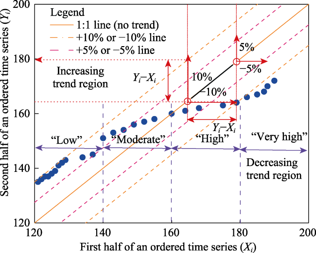
In this study, we applied an innovative trend analysis (ITA) technique to detect the annual and seasonal trends of solar photovoltaic resource potential (Rs) in East Asia during 1961-2010 based on the Global Energy Balance Archive (GEBA) data. The Mann-Kendall (M-K) trend test and linear regression method (LRM) were compared with the ITA technique. The results showed that the annual Rs in China presented a significant decreasing trend (D<-0.5 and P<0.01, where P is the P-value and D is the trend indicator of ITA) using these three techniques. The seasonal Rs generally showed a significant decreasing trend (D<-0.5) using the ITA technique in China, however, a slightly increasing trend was observed in Japan. The Rs values were further divided into four groups (“low”, “moderate”, “high” and “very high”) to detect the sub-trends using the ITA technique. The results indicated that the decreasing annual Rs in China was mainly due to reductions in the “high” and “very high” Rs values. The most probable causes of the trends in the variation in China were the decreasing sunshine duration and increasing anthropogenic aerosol loadings; while the trends in Japan were probably driven by the increasing sunshine and declining cloud optical thickness. Moreover, the similarities and differences between the M-K test and ITA technique results were compared and evaluated, and the ITA technique proved to be superior to the M-K test.

Cite this article

ZHOU Zhigao , HE Lijie , LIN Aiwen , WANG Lunche . Revisiting the Decadal Variability of Solar Photovoltaic Resource Potential in the Monsoon Climate Zone of East Asia Using Innovative Trend Analysis[J]. Journal of Resources and Ecology, 2023 , 14(6) : 1206 -1216 . DOI: 10.5814/j.issn.1674-764x.2023.06.009

1 Introduction

Global solar radiation/solar photovoltaic resource potential (Rs) reaching the Earth’s surface is the primary form of energy which contributes to many fields, such as the atmospheric environment, agricultural productivity and solar energy technologies (Mercado et al., 2009; Gray et al., 2010; Asaf et al., 2013; Wang et al., 2015; Del Hoyo et al., 2020). The solar photovoltaic (PV) installation capacity across China exceeded 175 GW in 2018, ranking first in the world (IRENA, 2019). Any changes in Rs can profoundly affect our lives and solar energy applications. For instance, Sweerts et al. (2019) estimated the losses of PV potential due to declining global solar radiation, and found that the PV potential decreased by 11%-15% from 1961 to 2015; and Zhou et al. (2021) found that the potential concentrated solar thermal power electricity production decreased by 136 kWh from 1961 to 2015 due to air pollution. Therefore, it is essential to obtain a clear understanding of the decadal variability of Rs for siting and evaluating solar energy systems in different parts of the world. At the global scale, Rs has decreased at many stations in past decades, however, increasing trends were also observed at some stations (Aksoy, 1997; Power, 2003; Nunez and Li, 2008; Takemura and Ohmura, 2009; Sanchez-Lorenzo et al., 2013). For example, Pinker et al. (2005) found that Rs had increased by 1.6 W m-2 decade-1 at the global scale from 1983 to 2001. Ruckstuhl et al. (2008) analyzed data from eight sites in Germany and Switzerland covering 1981 to 2005, and found an increasing trend of 2.6 W m-2 decade-1. Meanwhile, a decreasing trend of -8.6 W m-2 decade-1 was observed for a similar period (1981-2004) at 12 stations in India (Padma Kumari et al., 2007). Great uncertainties still exist in the accuracy of the variation trends of Rs at the global and regional scales, therefore, determining the decadal variability of Rs is particularly important for studies related to solar energy applications (Silva et al., 2010; Wild et al., 2013).
Many methods have been used to determine the decadal variability of meteorological and hydrological time series using various parametric and nonparametric methods, such as Sen’s Slope test, covariance analysis, Spearman’s Rho test, the Tramo/Seats program and the Mann-Kendall (M-K) test (Mann, 1945; Sen, 1968; Kendall, 1970; Haan, 2002). These techniques have been widely used for various meteorological and hydrological time series (Wu et al., 2008; Morin, 2011; Gebremicael et al., 2013). For example, Patra et al. (2012) used the Sen’s slope, linear regression method (LRM) and the M-K test to detect trends in rainfall over Orissa State, India during 1871-2006. The results showed insignificant negative trends in the variation for monsoon season and annual rainfall, but a positive trend in the post-monsoon season. Tabari et al. (2012) analyzed the trends of reference evaporation in Iran during 1966-2005 using the Spearman’s Rho and M-K tests, and found that significant increasing trends were observed at some stations. Sun et al. (2013) analyzed the trends of dissolved inorganic nitrogen (DIN) at three stations along the Yangtze River using the Tramo/Seats program during 1990-2009, and the results indicated that DIN was increasing at all stations. Guo et al. (2015) detected the trends of runoff and sediment in the upper reach of the Hanjiang River in China from 1956 to 2008 using the M-K test, and the results showed a decreasing trend since the 1990s. Wei and Deng (2014) determined the trend in the variation of precipitation in Xinjiang Chechen river basin during 1956-2008 using the M-K and SR tests, and a significant increasing trend was detected using these two methods.
Much progress has been made by applying various trend analysis techniques in the literature. However, parametric techniques (such as LRM and covariance analysis) require that the data are normally distributed or independent, which is inconsistent with the distributions of real-world hydrological or meteorological time series data (which tend to have positively or negatively skewed distributions). Non-parametric methods such as the M-K test, SR test, Sen’s Slope test and the Tramo/Seats program perform better in cases where the time series are considered as normal distributions and monotonic (Şen, 2012; Kisi, 2015), so some disadvantages still exist when applying these techniques to hydrological and meteorological time series data. Recently, an innovative trend analysis (ITA) technique was proposed by (Şen, 2012, 2014) and applied to various hydrological or meteorological time series analyses (Haktanir and Citakoglu, 2014; Ay and Kisi, 2015). For example, Ay and Kisi (2015) analyzed the trends of monthly precipitation using the ITA technique and the M-K test, and found that the ITA technique performed better than the M-K test in trend analysis (Kisi and Ay, 2014). Unfortunately, previous studies using the ITA technique mostly focused on the meteorological and hydrological time series, while most studies on Rs tended to apply various modeling methods (Pan et al., 2013; Amrouche and Le Pivert, 2014). For example, Deo et al. (2016) predicted the Rs using a wavelet-coupled support vector machine, and Chen et al. (2019) reconstructed a direct radiation dataset across China using different machine learning models. Few studies have examined the decadal variability of Rs around the world using different trend detection techniques, although a clear understanding of the variability of Rs at regional and global scales using various techniques is vitally significant due to its widespread application in the solar energy field (Kisi, 2015; Pashiardis et al., 2017). Due to its importance, a few experimental networks for the measurement of Rs have been established around the world, including Global Energy Balance Archive (GEBA), Baseline Surface Radiation Network (BSRN) and others, despite the great difficulties in conducting accurate observations (i.e., maintaining the sensor) and high cost (Qin et al., 2018). In China, a total of 122 stations are measuring global solar radiation, and the Rs data are available from the China meteorological administration (CMA) (Wang et al., 2015). However, previous studies have found that observed Rs data in China may have major inhomogeneity issues due to instrument replacement and sensitivity degradation (Wang et al., 2015).
Various decadal variability characteristics of Rs have been reported in different parts of East Asia. For instance, Hu et al. (2016) investigated the variability of PAR from 1961-2014 in the Tibetan plateau (TP) using estimated PAR values. The results showed that the variability of PAR in the TP showed an increasing trend from 1961 to 1983, an decreasing trend from 1983 to 2003 and then an increasing trend from 2003 to 2014, which is inconsistent with the known variability of PAR across China (Wang et al., 2016a). Xu et al. (2010) detected the variability of Rs at 16 stations in Northwest China during 1961-2007 using LRM, and 11 stations showed significant decreasing trends while no trends or slightly increasing trends were observed at the other five stations. Li et al. (2012) determined the decadal variability of Rs during 1961-2008 in South China and found that most stations showed significant decreasing trends. Wang and Wild (2016) analyzed the decadal variability of Rs across China, and found that Rs decreased across China in the dimming phase (1961-1989), while increasing Rs trends covered about two-thirds of China in the brightening phase (1993-2015). Zhou et al. (2019) investigated the decadal variability of Rs using homogenized Rs data and found that Rs showed an increasing trend of 0.92 W m-2 decade-1 during 1994-2015. Meanwhile, a generally increasing trend (of about +7 W m-2 decade-1) was observed from 1971-2002 in Japan (Norris and Wild, 2009). Since there is still no clear understanding of the decadal variability of Rs in China (Wang et al., 2016b) or Japan, this study applied a new approach, ITA, for the determination of Rs in East Asia.
The main objectives of this study are: 1) To analyze the decadal variability of Rs in East Asia using various trend detection techniques; 2) To compare and evaluate the advantages, similarities and differences of the ITA technique and the M-K test at different stations; and 3) To discuss the decadal variability of Rs in East Asia and its possible causes.

2 Materials and methods

2.1 Study area and data

The study area is East Asia, including Japan, China, South Korea, Mongolia, and North Korea, facing to the Pacific Ocean on the east. Figure 1 shows the geographical locations of the Sapporo, Tateno, Kumamoto, Harbin, Shenyang, Beijing, Wuhan and Guangzhou stations used in this study. East Asia is the world’s most typical monsoon climate region. For example, Harbin station is located in the temperate continental monsoon climatic zone, and the annual mean rainfall and mean air temperatures in summer and winter are about 569.1 mm, 23 ℃ and -19℃, respectively. Guangzhou station is characterized by the oceanic subtropical monsoon climate, where the mean temperature of the hottest month is in July (28 ℃) and the mean temperature of coldest month is in January (9-16 ℃). The Rs monthly data from these eight stations across East Asia were provided by the Global Energy Balance Archive (GEBA), which is a database maintained and developed by the institute for atmospheric and climate science at ETH Zurich, Switzerland. This data has been used in various research applications, such as the estimation of long-term trends in Rs (Wild et al., 2005; Wild, 2009). In this study, an annual mean Rs value was obtained for each month of the year from the total data series across all years, and all further computations were based on these annual mean Rs values. In cases where less than two missing or incorrect annual mean Rs values occurred at one station, interpolation was used to fill in the missing values or replace the incorrect values. Otherwise, the data for that station were used as detected. Moreover, if less than 45 continuous-year measured data points were available at a station, that station was eliminated in order to study the decadal variability of Rs. Ultimately, eight stations were selected from the GEBA database based on the completeness of records, the spatial distribution of the station and the length of the recorded history. The qualified records mostly began in the year 1961 and ended in 2010. The detailed information about the stations (i.e., codes, station names and elevations) and radiation data are shown in Table 1.
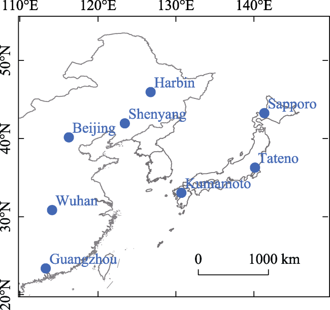
Fig. 1 Distribution of the eight stations in East Asia
Table 1 Geographical information for the stations and record period of the Rs time series data
Code Station name Elevation (m) Record period Record length (yr)
880 Sapporo 17 1958-2010 53
886 Tateno 25 1958-2007 50
2685 Kumamoto 38 1961-2007 47
2039 Harbin 142 1961-2010 50
2041 Shenyang 43 1961-2010 50
2042 Beijing 55 1958-2010 53
2046 Wuhan 23 1961-2010 50
2048 Guangzhou 7 1961-2010 50

2.2 Methodology

2.2.1 The linear regression method and Mann-Kendall (M-K) test

The linear regression method (LRM) is a classical technique that can be used to detect the decadal variability of various types of time series at different scales (Tabari and Talaee, 2011). The non-parametric M-K test, proposed by Mann (1945) and Kendall (1970), has been widely applied to determining the trends in the variation of time series and evaluate the significance of trends in various meteorological and hydrologic time series (Zhou et al., 2018).

2.2.2 Innovative trend analysis

The innovative trend analysis (ITA) proposed by (Şen, 2012) has been widely applied in various meteorological and hydrologic time series studies (Zhou et al., 2018). In this method, a time series is first divided into two equal halves (sub-series) from the first date to the last date. Then both sub-series are sorted in ascending order. Finally, the first half series (Xi : i = 1, 2,…, n/2) is located on the X-axis and the second half series (Yj: j = n/2+1, n/2+2,…, n) is placed on the Y-axis of the Cartesian coordinate system (Fig. 2). If the two sub-series are equal, the points will be aggregated on the 1:1 (45°) line in the scatter plot, which indicates no trend; if the points fall above the 1:1 line, the time series shows an increasing trend; and if the points accumulate below the 1:1 line, it means that the time series shows a decreasing trend (Şen, 2012, 2014). Meanwhile, one innovation is to divide Rs into four groups (low, moderate, high and very high groups) according to the Rs values, as shown in Fig. 2. The quantitative selection of group boundaries differs from one station to another, and such a plot provides the first visual inspection of the various types of sub-trends (Dabanlı et al., 2016). Meanwhile, the ITA slope is expressed according to the following equation (Şen, 2015):
$S=\frac{2\times \left( {{{\bar{y}}}_{2}}-{{{\bar{y}}}_{1}} \right)}{n}$
where ${{\bar{y}}_{1}}$ and ${{\bar{y}}_{2}}$ are the arithmetic means of the first and the second sub-series, respectively; n denotes the number of data; and S is the ITA slope.
Fig. 2 Illustration of the ITA method
Wu and Qian (2017) improved the algorithm that identified trends using ITA. The ITA trend indicator D is calculated as follows:
$D=\frac{1}{n}\underset{i=1}{\overset{n}{\mathop{\mathop{\sum }^{}}}}\,\frac{10\times \left( {{y}_{i}}-{{x}_{i}} \right)}{{\bar{x}}}$
where $\bar{x}$ is the arithmetic mean of the first sub-series, n is the number of data points; and xi and yi are the i-th observations of the first and second sub-series, respectively. As the trend detection is based on the first sub-series, the trend indicator D is derived from the mean difference divided by the mean of the first sub-series. A positive value of D indicates an increasing trend, whereas a negative value indicates a decreasing trend. Therefore, a rising or falling trend is very significant when all the points fall above the line at +10% above or -10% below the line, i.e., |D| > 1. When all the points accumulate between +5% and +10% or between -5% and -10%, then 0.5< |D| <1, and this value indicates that a rising or falling trend is significant. When all the points are collected between +2% and +5% or between −2% and -5%, then 0.2< |D| <0.5, and this value indicates a slight trend. When all points fall between +2% and -2%, then |D| < 0.2, which indicates that the points are very close to the 1:1 (45°) line, so almost no trend is observed.

3 Results and discussion

Figure 3a shows the distribution of the annual mean Rs at the eight stations in East Asia. The values ranged from 130 W m-2 to 170 W m-2, which indicated that the annual mean Rs at these stations in East Asia exhibited large differences. While outliers were observed at the eight stations (ranging from 93 W m-2 to 194 W m-2), most of them were only mild outliers, meaning that the differences between the average values of the time series and the outliers were not more than three times the standard deviation of the time series. This finding suggested that the Rs data after quality control was reliable. Figure 3b shows the monthly mean Rs in Beijing station (as an example), where the mean radiation values in spring, summer, autumn and winter were 211, 213, 139 and 106 W m-2, respectively. The high values of Rs were mostly distributed in spring and summer, accounting for more than 60% of the Rs in the whole year.
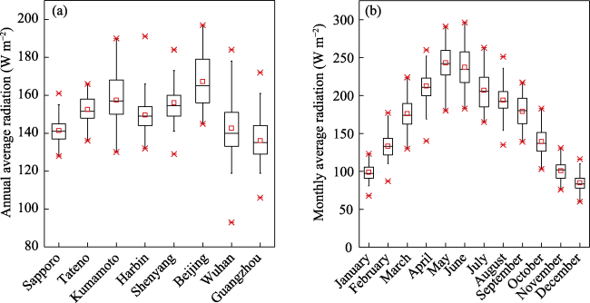
Fig. 3 Boxplots of (a) annual mean Rs at the eight stations in East Asia, and (b) monthly mean Rs at the Beijing station. The boxes indicate the 25th, 50th, and 75th percentiles. The ends of the whiskers indicate the lowest (highest) datum within 1.5 times the interquartile range of the lower (upper) quartile

3.1 Annual trends

The variability in annual Rs determined using the three above techniques (four statistics) are shown in Table 2. Obvious differences in the trend variations of Rs are evident at the different station. The values of D (trend slope) at four stations in China (Shenyang, Beijing, Wuhan and Guangzhou) were -0.54, -1.29, -1.07 and -0.75, respectively. The Z and b values were all significant negative values (P< 0.01) at those four stations. The Beijing, Shenyang, Wuhan and Guangzhou stations showed decreasing trends at rates of -7.7 W m-2 decade-1, -3.5 W m-2 decade-1, -6.1 W m-2 decade-1 and -4.1 W m-2 decade-1, respectively (P< 0.01). This finding indicated that the Rs decreased significantly at these stations during 1961-2010 using the three methods. However, the decadal variability of Rs at the Sapporo, Tateno, Kumamoto and Harbin stations were not found to be significantly decreasing (P>0.1 and |D| <0.2) using the three methods, except that an increasing trend (P<0.1) at Kumamoto station was observed using the M-K test.
Table 2 Values of different statistics indicators for LRM, M-K test and ITA method
Station name b Z S D
Annual Low Moderate High Very high
Sapporo 0.02 0.17 -0.01 -0.03 -0.09 -0.04 0.02 -0.01
Tateno 0.06 1.09 0.04 0.07 -0.15 0.01 0.16 0.22
Kumamoto 0.12 1.80* 0.07 0.11 0.27 -0.02 0.15 0.06
Harbin -0.11 -1.61 -0.03 -0.05 -0.12 -0.22 -0.19 0.30
Shenyang -0.35*** -2.66*** -0.35 -0.54 -0.30 -0.20 -0.45 -1.12
Beijing -0.77*** -6.04*** -0.89 -1.29 -0.88 -1.12 -1.50 -1.65
Wuhan -0.61*** -2.79*** -0.65 -1.07 -0.69 -0.40 -1.01 -2.04
Guangzhou -0.41*** -3.31*** -0.42 -0.75 -0.70 -0.58 -0.71 -0.97

Note: * indicates significant trend at 10% significant level, ** indicates significant trend at 5% significant level, and *** indicates significant trend at 1% significant level. b is the slope of LRM, Z donates the standard normal test statistics of M-K test, S represents the slope of ITA, and D means the slope of ITA for the low, moderate, high and very high groups. The same below.

The sub-trends of annual Rs in the four groups detected by ITA are presented in Table 2. The results showed that the D values were mostly negative at the eight stations, and the values of D for the “very high” group at the Shenyang, Beijing, Wuhan, and Guangzhou stations in China were -1.12, -1.65, -2.04 and -0.97, respectively. Meanwhile, the values of D were unequal across the different Rs groups at each station, and sometimes even opposite in sign. The values of D decreased gradually at the four stations in China (Beijing, Shenyang, Wuhan, and Guangzhou), ranging from “low” to “very high” Rs values. This result showed that the higher the Rs, the larger the trend values, which indicated that the reductions of Rs in China were mainly due to the reductions in the “high” and “very high” Rs values during 1961-2010 at the four stations. In the “high” and “very high” groups, the impacts of clouds on the Rs would be relatively smaller and the aerosol impact would be larger, compared with the “low” and “moderate” groups. Therefore, this provides preliminary evidence that aerosol was the leading factor influencing Rs in China. In general, the ITA results (Fig. 4) showed that most points in China fall below the 1:1 line, suggesting an overall decreasing trend for the four groups. Most points in Japan accumulate above the 1:1 line, suggesting a slightly increasing trend or no trend in the four groups in Japan.
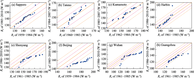
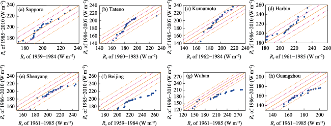
Fig. 4 Results of ITA for the annual Rs at the eight stations in East Asia

Note: The dot in the figure is the global solar radiation (Rs) value. The same below.

The above analysis revealed that a significant decreasing trend of more than -3.5 W m-2 decade-1 (P<0.01 and D < -0.5) was observed for Rs in China (except at Harbin station) and a slightly increasing trend of 1.2 W m-2 decade-1 was observed in Japan during 1961-2010. A large amount of fossil fuel was burned to develop the economy rapidly in China, resulting in increasing anthropogenic aerosol loadings during the past decades (Wang and Shi, 2010). The increases in anthropogenic aerosol loadings would result in reductions in direct radiation, leading to the reductions in Rs. Some other natural factors influencing the decadal variability of Rs have also been analyzed, such as the reductions in sunshine duration in China during the past decades (Ren et al., 2005; Li et al., 2013). Yu et al. (2011) analyzed the decadal variability of sunshine duration at 194 stations in China during 1951-2009, and found a significant decreasing trend (-36.9 h decade-1). The main reason why Rs showed no trends or slightly increasing trends at the three stations in Japan may have been the increasing sunshine duration (+23 h decade-1) during the 20th century, especially since the mid-1980s (Stanhill and Cohen, 2008). Meanwhile, the increases in atmospheric transparency and reductions in cloud optical thickness from 1974 to 2006 might also partly explain the increasing Rs in Japan (Tsutsumi and Murakami, 2012). Moreover, aerosol optical depth had decreased by 0.02 to 0.75 μm at 14 stations (including Sapporo and Tateno stations) from 1970 to 2000; therefore, the solar brightening in Japan could be attributed to the reduction in aerosol optical depth (Kudo et al., 2012).
However, the decadal variability of Rs in the four different groups using ITA differed greatly at each station. There were no significant trends in the four different Rs groups at the three stations in Japan (Fig. 4a-c ), except that slightly increasing trends were detected for “very high” Rs values at Tateno station and “low” Rs values at Kumamoto station (the values of D were 0.22 and 0.27, respectively). At Harbin station (Fig. 4d), the “low”, “moderate” and “high” Rs groups decreased slightly, and the values of D were -0.12, -0.22 and -0.19, respectively, however, the “very high” Rs group showed an increasing trend and the value of D was 0.3. The “low”, “moderate” and “high” Rs groups showed slightly decreasing trends at Shenyang station (Fig. 4e), the values of D were -0.3, -0.2 and -0.45, respectively, and the “very high” Rs group showed a significant decreasing trend. Fig. 4f and Fig. 4h generally showed decreasing trends of more than 5% in all Rs groups at Beijing and Guangzhou stations. Fig. 4g shows a rapidly decreasing trend (less than -20%) for “very high” radiation values at Wuhan station, and the value of D was -2.04.

3.2 Seasonal trends

The trends in Rs variation at each station for the four seasons detected by the above methods (four statistics) are summarized in Table 3. The Rs in spring showed significant decreasing trends (P<0.01) using the M-K test at the Shenyang and Beijing stations. However, there were significant decreasing trends (D<-0.5) at the Shenyang, Beijing, Wuhan and Guangzhou stations in China using ITA, which indicated that some trends that could not be detected by the M-K test could be identified effectively using the ITA technique.
Table 3 Values of slope b of the LRM, Z of the M-K test, and S and D of ITA for Rs in spring, summer, autumn, and winter
Season Value Sapporo Tateno Kumamoto Harbin Shenyang Beijing Wuhan Guangzhou
Spring b -0.08 -0.03 0.06 -0.11 -0.64*** -0.78*** -0.22 -0.42**
Z -0.78 -0.47 1.61 -1.41 -3.65*** -4.99*** -0.26 -1.31
S -0.07 -0.15 0.03 0.03 -0.51 -0.95 -0.32 -0.38
D -0.09 -0.19 0.03 0.04 -0.63 -1.11 -0.52 -0.80
Summer b -0.03 0.02 0.12 0.08 -0.32** -0.98*** -1.21*** -0.47***
Z 0.48 0.60 1.07 0.51 -1.79* -5.63*** -3.70*** -2.63***
S 0.01 0.07 0.20 0.16 -0.41 -1.16 -1.26 -0.54
D 0.02 0.09 0.24 0.20 -0.49 -1.32 -1.44 -0.78
Autumn b 0.02* 0.15 -0.02 -0.18* -0.28** -0.68*** -0.42** -0.39***
Z 0.82 1.90** 1.13 -1.46 -2.06** -5.78*** -2.43** -2.35**
S -0.02 0.11 0.05 -0.08 -0.34 -0.82 -0.44 -0.46
D -0.05 0.22 0.08 -0.18 -0.63 -1.42 -0.80 -0.72
Winter b 0.05 0.09 -0.04 -0.25*** -0.19*** -0.50*** -0.57*** -0.33**
Z 1.28 0.81 -0.15 -3.69*** -1.81* -5.33*** -3.72*** -1.71*
S 0 0.12 0.04 -0.24 -0.16 -0.60 -0.55 -0.29
D 0.02 0.26 0.09 -0.74 -0.42 -1.37 -1.44 -0.64
The Rs in summer (Fig. 5) showed significant decreasing trends using the M-K test and LRM at the Shenyang, Beijing, Wuhan and Guangzhou stations in China. Meanwhile, significant decreasing trends were detected using ITA at those four stations, and the values of D were -0.49, -1.32, -1.44 and -0.78, respectively. These results indicated that the ITA method was in good agreement with the M-K test and LRM. Moreover, the Kumamoto and Harbin stations showed slightly increasing trends, with D values of 0.24 and 0.2, respectively.
Fig. 5 Results of ITA for Rs in summer in East Asia
The Rs in autumn exhibited significant trends using the M-K test and LRM at all stations, except for the Kumamoto station (Table 3). The four stations in China showed significant decreasing trends using ITA, and the values of D were -0.63, -1.42, -0.8 and -0.72, respectively (Table 3). A slightly increasing trend (D = 0.22) was also observed using ITA at Tateno station in Japan (Table 3).
The Rs in winter showed significant decreasing trends using the M-K test and LRM at Harbin, Shenyang, Beijing, Wuhan and Guangzhou stations in China (Table 3). Four stations in China (Harbin, Beijing, Wuhan, and Guangzhou) showed significant or very significant decreasing trends using ITA, and the values of D (trend slope) were -0.74, -1.37, -1.44 and -0.64, respectively (Table 3). Meanwhile, a slightly increasing trend (D = 0.26) was observed using ITA at the Tateno station (Table 3).
The above analysis revealed that there was a significant decreasing trend in China and a slightly increasing trend in Japan for Rs in the four different seasons during 1961-2010. Sunshine duration showed a significant decreasing trend in all four seasons in China, directly leading to the reductions of Rs in China (Yu et al., 2011). The lack of trends or slightly increasing trends observed at the three stations in Japan were possibly due to the decreasing aerosol optical depth (Kudo et al., 2010). The trend in the annual variation of Rs at Harbin station was insignificant, which could be explained by the opposite trends in summer and winter. In other words, a significant decreasing trend (D = -0.74) was observed in winter, however, a slightly increasing trend (D = 0.2) was observed in summer at Harbin station.

3.3 Comparison of the three trend analysis methods

The results of the 40 time series trend analyses above are summarized in Table 4. Significant trends (P<0.05) were observed in 20 series using LRM, and 17 series using the M-K test. The ITA method generally presented similar results, i.e., 24 series (including the above 20 series) showed decreasing or increasing trends of more than 2%, 18 series showed decreasing or increasing trends of more than 5% and 10 series showed decreasing trends of more than 10%, which indicated high levels of agreement in the trends of variation among these methods. The high level of agreement among the methods demonstrated that the ITA method was effective for determining the trends in Rs in East Asia. Meanwhile, the ITA method showed many advantages. For example, it does not have any assumptions (e.g., sample number, non-normality, serial correlation, etc.) unlike the M-K method. Another advantage is that the variation trends of different groups (“low”, “moderate”, “high” and “very high” values) can be easily determined using the ITA technique.
Table 4 Comparisons of the test results using the LRM, M-K and ITA techniques
Station Season Linear regression Mann-Kendall ITA method
Sapporo Annual No No No
Spring No No No
Summer No No No
Autumn No No No
Winter No No No
Tateno Annual No No No
Spring No No No
Summer No No No
Autumn No * *
Winter No No *
Kumamoto Annual No No No
Spring No No No
Summer No No No
Autumn No No No
Winter No No No
Harbin Annual No No No
Spring No No No
Summer No No *
Autumn No No No
Winter * ** **
Shenyang Annual ** ** ***
Spring ** ** **
Summer * No *
Autumn * * **
Winter ** No *
Beijing Annual ** ** ***
Spring ** ** ***
Summer ** ** ***
Autumn ** ** ***
Winter ** ** ***
Wuhan Annual ** ** ***
Spring No No **
Summer ** ** ***
Autumn * * **
Winter ** ** ***
Guangzhou Annual ** ** ***
Spring * No **
Summer ** ** **
Autumn ** * **
Winter * No **

Note: No indicates no significant trend at 5% significant level (or 2% trend line); * indicates significant trend at 5% significant level (or 2% trend line); ** indicates significant trend at 1% significant level (or 5% trend line); and *** indicates significant trend at 10% trend line.

4 Conclusions

The ITA technique was used to detect trends in the annual and seasonal variations in Rs in East Asia, and two commonly used techniques, i.e., LRM and the M-K test, were also used to evaluate the reliability of ITA in this study. As a graphical method, ITA presented the results intuitively, and the trends of variations in different groups can be obtained. The conclusions are threefold.
(1) Most stations in China (except for Harbin) showed significant decreasing trends (P<0.01) at a rate of -3.5 W m-2 decade-1 using LRM and the M-K test for annual Rs. The values of D for different Rs groups using ITA were not usually equal to those of the overall Rs, and occasionally they were even opposite in sign, such as the “moderate” and “very high” groups at Harbin station. The values of average D in different Rs groups indicated that the decreasing Rs levels in China were mainly due to reductions in the “high” and “very high” Rs groups, preliminarily indicating that aerosol was the leading factor influencing the Rs in China.
(2) Detecting the trends in the seasonal and annual variations of Rs using the ITA technique, Shenyang, Beijing, Wuhan and Guangzhou stations in China showed significant decreasing trends (D<-0.5) in all four seasons. However, Kumamoto and Harbin stations showed increasing trends in summer. Tateno station also presented increasing trends in autumn and winter. Therefore, a significant decreasing trend for Rs was identified in China, while a slightly increasing trend was observed in Japan. The increases of anthropogenic aerosol loadings and reductions in sunshine duration in China during the past decades may have contributed to these results. The trends in the variations of Rs in Japan might be due to the increasing sunshine duration and atmospheric transparency, and the reductions in aerosol optical depth in Japan since the middle of the 1980s.
(3) The results from the ITA method were in good agreement with LRM and the M-K test. Meanwhile, some trends that could not be detected by the M-K test could be effectively found using the ITA technique.
Overall, the ITA technique exhibited many advantages. Firstly, the ITA technique made it easy to calculate the slope. Secondly, the ITA technique could be applied to various types of time series without considering the seasonal cycle, the size of data or the distribution assumption in the serial correlation. Thirdly, one feature of the ITA technique was its ability to detect different groups (“low”, “moderate”, “high” and “very high” values) of a time series in a Cartesian coordinate system. Thus, this feature helped in detecting hidden sub-trends that could be observed easily because of the graphical presentation of the results.
This study comprehensively determined the dacadal variability of Rs at eight stations in East Asia during 1961-2010. The results will contribute to many fields, such as energy applications, the atmospheric environment and climate prediction. This study represents the first application of the ITA method in the field of solar energy for accurately determining the radiation variations at a regional scale, which also lays the foundations for other research fields, including environmental evolution and energy utilization. Meanwhile, this was just a preliminary attempt to discuss the Rs variations using different trend detection techniques, and the effects of water vapor and cloud-aerosol interactions also warrant further analysis in our future work.

Acknowledgement

The global solar radiation (Rs) data from 1961 to 2010 in China and Japan in this study were obtained from the Global Energy Balance Archive (GEBA), which was highly appreciated by the authors.
[1]
Aksoy B. 1997. Variations and trends in global solar radiation for Turkey. Theoretical and Applied Climatology, 58(1): 71-77.

DOI

[2]
Amrouche B, Le Pivert X. 2014. Artificial neural network based daily local forecasting for global solar radiation. Applied Energy, 130: 333-341.

DOI

[3]
Asaf D, Rotenberg E, Tatarinov F, et al. 2013. Ecosystem photosynthesis inferred from measurements of carbon sulphide flux. Nature Geoscience, 6(3): 186-190.

DOI

[4]
Ay M, Kisi O. 2015. Investigation of trend analysis of monthly total precipitation by an innovative method. Theoretical and Applied Climatology, 120(3): 617-629.

DOI

[5]
Chen F Y, Zhou Z G, Lin A W, et al. 2019. Evaluation of direct horizontal irradiance in China using a physically-based model and machine learning methods. Energies, 12(1): 150. DOI: 10.3390/en12010150.

[6]
Dabanlı İ, Şen Z, et al.Yeleğen M Ö, 2016. Trend assessment by the innovative Şen method. Water Resources Management, 30(14): 5193-5203.

DOI

[7]
del Hoyo M, Rondanelli R, Escobar R. 2020. Significant decrease of photovoltaic power production by aerosols. The case of Santiago de Chile. Renewable Energy, 148: 1137-1149.

DOI

[8]
Deo R C, Wen X H, Qi F. 2016. A wavelet-coupled support vector machine model for forecasting global incident solar radiation using limited meteorological dataset. Applied Energy, 168: 568-593.

DOI

[9]
Gebremicael T G, Mohamed Y A, Betrie G D, et al. 2013. Trend analysis of runoff and sediment fluxes in the Upper Blue Nile Basin: A combined analysis of statistical tests, physically-based models and landuse maps. Journal of Hydrology, 482: 57-68.

DOI

[10]
Gray L J, Beer J, Geller M, et al. 2010. Solar influences on climate. Reviews of Geophysics, 48(4): RG4001. DOI: 10.1029/2009RG000282.

[11]
Guo S X, Liu B, Wang G S, et al. 2015. Trend analysis of flow and sediment in upstream of Hanjiang Basin based on Mann-Kendall test method. Water Resources and Power, 33(11): 140-142. (in Chinese)

[12]
Haan C T. 2002. Statistical methods in hydrology. Ames, USA: Iowa State University Press.

[13]
Haktanir T, Citakoglu H. 2014. Trend, independence, stationarity, and homogeneity tests on maximum rainfall series of standard durations recorded in Turkey. Journal of Hydrologic Engineering, 19(9): 0000973. DOI: 10.1061/(ASCE)HE.1943-5584.0000973.

[14]
Hu B, Liu H, Wang Y S. 2016. Investigation of the variability of photosynthetically active radiation in the Tibetan Plateau, China. Renewable and Sustainable Energy Reviews, 55: 240-248.

DOI

[15]
IRENA. 2019. Renewable energy statistics 2019. Abu Dhabi, The United Arab Emirates: The International Renewable Energy Agency.

[16]
Kendall M G. 1970. Rank correlation methods. London, UK: Griffin.

[17]
Kisi O, Ay M. 2014. Comparison of Mann-Kendall and innovative trend method for water quality parameters of the Kizilirmak River, Turkey. Journal of Hydrology, 513: 362-375.

DOI

[18]
Kisi O. 2015. An innovative method for trend analysis of monthly pan evaporations. Journal of Hydrology, 527: 1123-1129.

DOI

[19]
Kudo R, Uchiyama A, Ijima O, et al. 2012. Aerosol impact on the brightening in Japan. Journal of Geophysical Research: Atmospheres, 117: D07208. DOI: 10.1029/2011JD017158.

[20]
Kudo R, Uchiyama A, Yamazaki A, et al. 2010. From solar radiation measurements to optical properties: 1998-2008 trends in Japan. Geophysical Research Letters, 37(4): L04805. DOI: 10.1029/2009GL041794.2010.

[21]
Li H Q, Fu Z T, Wen X Y, et al. 2013. Characteristic analysis of sunshine duration change in China during the last 50 years. Climatic and Environmental Research, 18(2): 203-209. (in Chinese)

[22]
Li Y L, He R, Du Y D. 2012. Spatiotemporal variation characteristics of total solar radiation in South China region. Renewable Energy Resources, 30(1): 13-16. (in Chinese)

[23]
Mann H B. 1945. Nonparametric tests against trend. Econometrica, 13(3): 245-259.

DOI

[24]
Mercado L M, Bellouin N, Sitch S, et al. 2009. Impact of changes in diffuse radiation on the global land carbon sink. Nature, 458(7241): 1014-1017.

DOI

[25]
Morin E. 2011. To know what we cannot know: Global mapping of minimal detectable absolute trends in annual precipitation. Water Resources Research, 47(7): W07505. DOI: 10.1029/2010WR009798.

[26]
Norris J R, Wild M. 2009. Trends in aerosol radiative effects over China and Japan inferred from observed cloud cover, solar “dimming,” and solar “brightening”. Journal of Geophysical Research: Atmospheres, 114: D00D15. DOI: 10.1029/2008JD011378.

[27]
Nunez M, Li Y. 2008. A cloud-based reconstruction of surface solar radiation trends for Australia. Theoretical and Applied Climatology, 91(1): 59-75.

DOI

[28]
Padma Kumari B, Londhe A L, Daniel S, et al. 2007. Observational evidence of solar dimming: Offsetting surface warming over India. Geophysical Research Letters, 34(21): L21810. DOI: 10.1029/2007GL031133.

[29]
Pan T, Wu S H, Dai E F, et al. 2013. Estimating the daily global solar radiation spatial distribution from diurnal temperature ranges over the Tibetan Plateau in China. Applied Energy, 107: 384-393.

DOI

[30]
Pashiardis S, Kalogirou S A, Pelengaris A. 2017. Statistical analysis for the characterization of solar energy utilization and inter-comparison of solar radiation at two sites in Cyprus. Applied Energy, 190: 1138-1158.

DOI

[31]
Patra J P, Mishra A, Singh R, et al. 2012. Detecting rainfall trends in twentieth century (1871-2006) over Orissa State, India. Climatic Change, 111(3): 801-817.

DOI

[32]
Pinker R T, Zhang B, Dutton E G. 2005. Do satellites detect trends in surface solar radiation? Science, 308(5723): 850-854.

PMID

[33]
Power H C. 2003. Trends in solar radiation over Germany and an assessment of the role of aerosols and sunshine duration. Theoretical and Applied Climatology, 76(1): 47-63.

DOI

[34]
Qin W M, Wang L C, Lin A W, et al. 2018. Comparison of deterministic and data-driven models for solar radiation estimation in China. Renewable and Sustainable Energy Reviews, 81: 579-594.

DOI

[35]
Ren G Y, Guo J, Xu M Z, et al. 2005. Climate changes of China’s mainland over the past half century. Acta Meteorologica Sinica, 63(6): 942-956. (in Chinese)

[36]
Ruckstuhl C, Philipona R, Behrens K, et al. 2008. Aerosol and cloud effects on solar brightening and the recent rapid warming. Geophysical Research Letters, 35: L12708. DOI: 10.1029/2008GL034228.

[37]
Sanchez-Lorenzo A, Calbó J, Wild M. 2013. Global and diffuse solar radiation in Spain: Building a homogeneous dataset and assessing their trends. Global and Planetary Change, 100: 343-352.

DOI

[38]
Sen P K. 1968. Estimates of the regression coefficient based on Kendall’s tau. Journal of the American Statistical Association, 63(324): 1379-1389.

DOI

[39]
Şen Z. 2012. Innovative trend analysis methodology. Journal of Hydrologic Engineering, 17(9): 1042-1046.

DOI

[40]
Şen Z. 2014. Trend identification simulation and application. Journal of Hydrologic Engineering, 19(3): 635-642.

DOI

[41]
Şen Z. 2015. Innovative trend significance test and applications. Theoretical and Applied Climatology, 127(3): 939-947.

DOI

[42]
Silva V D P R D, Silva R A E, Cavalcanti E P, et al. 2010. Trends in solar radiation in NCEP/NCAR database and measurements in northeastern Brazil. Solar Energy, 84(10): 1852-1862.

[43]
Stanhill G, Cohen S. 2008. Solar radiation changes in Japan during the 20th century: Evidence from sunshine duration measurements. Journal of the Meteorological Society of Japan Ser II, 86(1): 57-67.

DOI

[44]
Sun C C, Shen Z Y, Xiong M, et al. 2013. Trend of dissolved inorganic nitrogen at stations downstream from the Three-Gorges Dam of Yangtze River. Environmental Pollution, 180: 13-18.

DOI PMID

[45]
Sweerts B, Pfenninger S, Yang S, et al. 2019. Estimation of losses in solar energy production from air pollution in China since 1960 using surface radiation data. Nature Energy, 4(8): 657-663.

DOI

[46]
Tabari H, Nikbakht J, Talaee P H. 2012. Identification of trend in reference evapotranspiration series with serial dependence in Iran. Water Resources Management, 26(8): 2219-2232.

DOI

[47]
Tabari H, Talaee P H. 2011. Temporal variability of precipitation over Iran: 1966-2005. Journal of Hydrology, 396(3-4): 313-320.

DOI

[48]
Takemura T, Ohmura A. 2009. Trend of surface solar radiation over Asia simulated by aerosol transport-climate model. San Francisco, USA: AGU Fall Meeting.

[49]
Tsutsumi Y, Murakami S. 2012. Increase in global solar radiation with total cloud amount from 33 years observations in Japan. Journal of the Meteorological Society of Japan Ser II, 90(4): 575-581.

DOI

[50]
Wang B, Shi G Y. 2010. Long-term trends of atmospheric absorbing and scattering optical depths over China region estimated from the routine observation data of surface solar irradiances. Journal of Geophysical Research: Atmospheres, 115: D00K28. DOI: 10.1029/2009JD013239.

[51]
Wang K C, Ma Q, Li Z J, et al. 2015. Decadal variability of surface incident solar radiation over China: Observations, satellite retrievals, and reanalyses. Journal of Geophysical Research: Atmospheres, 120(13): 6500-6514.

[52]
Wang L C, Kisi O, Zounemat-Kermani M, et al. 2016a. Modeling and comparison of hourly photosynthetically active radiation in different ecosystems. Renewable and Sustainable Energy Reviews, 56: 436-453.

DOI

[53]
Wang L C, Kisi O, Zounemat-Kermani M, et al. 2016b. Solar radiation prediction using different techniques: Model evaluation and comparison. Renewable and Sustainable Energy Reviews, 61: 384-397.

DOI

[54]
Wang Y W, Wild M. 2016. A new look at solar dimming and brightening in China. Geophysical Research Letters, 43(22): 11777-11785.

[55]
Wei G H, Deng L J. 2014. Analysis on precipitation trend in arid regions based on non-parametric verification methods of Mann-Kendall and Spearman’s rho. Northwest Hydropower, (4): 1-4. (in Chinese)

[56]
Wild M. 2009. Global dimming and brightening: A review. Journal of Geophysical Research, 114: D00D16. DOI: 10.1029/2008JD011470.

[57]
Wild M, Folini D, Schär C, et al. 2013. The global energy balance from a surface perspective. Climate Dynamics, 40(11): 3107-3134.

DOI

[58]
Wild M, Gilgen H, Roesch A, et al. 2005. From dimming to brightening: Decadal changes in solar radiation at Earth’s surface. Science, 308(5723): 847-850.

DOI

[59]
Wu H, Qian H. 2017. Innovative trend analysis of annual and seasonal rainfall and extreme values in Shaanxi, China, since the 1950s. International Journal of Climatology, 37(5): 2582-2592.

DOI

[60]
Wu H, Soh L K, Samal A, et al. 2008. Trend analysis of streamflow drought events in Nebraska. Water Resources Management, 22(2): 145-164.

DOI

[61]
Xu J M, He J H, Yan F X. 2010. Research on secular variation of solar radiation over northwest China from 1961 to 2007. Climatic and Environmental Research, 15(1): 89-96. (in Chinese)

[62]
Yu H Y, Liu S H, Zhao N, et al. 2011. Variation characteristics of the sunshine duration and its relationships with temperature, wind speed, and precipitation over recent 59 years in China. Climatic and Environmental Research, 16(3): 389-398. (in Chinese)

[63]
Zhou Z G, Lin A W, Qin W M, et al. 2019. Trends in downward surface shortwave radiation from multi-source data over China during 1984-2015. International Journal of Climatology, 40(13): 3467-3485.

DOI

[64]
Zhou Z G, Lin A W, Wang L C, et al. 2021. Estimation of the losses in potential concentrated solar thermal power electricity production due to air pollution in China. Science of the Total Environment, 784: 147214. DOI: 10.1016/j.scitotenv.2021.147214.

[65]
Zhou Z G, Wang L C, Lin A W, et al. 2018. Innovative trend analysis of solar radiation in China during 1962-2015. Renewable Energy, 119: 675-689.

DOI

Outlines

/