Resource and Environment

Green Water Resource Utilization Efficiency in Urban Agglomerations: Measurement, Spatiotemporal Variations and Influencing Factors

  • HU Mianhao , 1, * ,
  • CHEN La 2 ,
  • YUAN Juhong 3
Expand
  • 1. School of Economics, Jiangxi University of Finance & Economics, Nanchang 330032, China
  • 2. Institute of Ecological Civilization, Jiangxi University of Finance & Economics, Nanchang 330032, China
  • 3. College of Art, Jiangxi University of Finance and Economics, Nanchang 330032, China
* HU Mianhao, E-mail:

Received date: 2022-09-06

  Accepted date: 2023-01-30

  Online published: 2023-10-23

Supported by

The Science and Technology Projects of Jiangxi Provincial Education Department(GJJ2200518)

The Ministry of Education in China of Humanities and Social Sciences(20YJAZH037)

Abstract

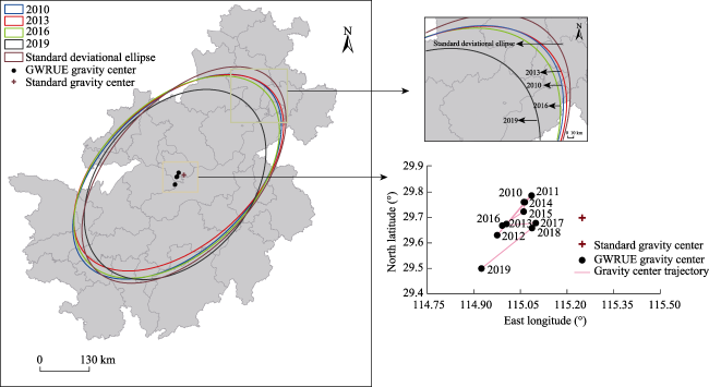
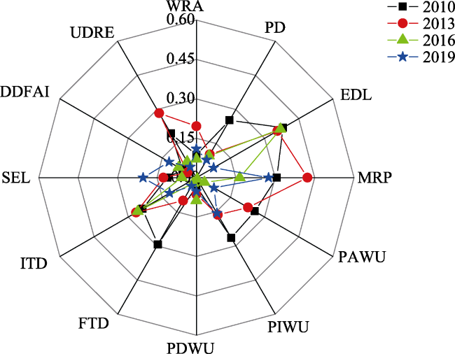
Green development is the coordinated development of the economy, society and environment and has become a mainstream development model. This paper evaluates the green water resource utilization efficiency (GWRUE) of 38 regions in the four-city area in central China during 2010-2019 using a super-slacks-based measure (super-SBM) DEA model considering unexpected output. Then, the spatiotemporal variations in GWRUE are analyzed by the standard deviational ellipse method, and the geographical detector method is employed to reveal the dominant impacts and interaction impacts on GWRUE spatiotemporal variations. The results show that: (1) From 2010 to 2019, the GWRUE in the four-city area in central China was low, and the difference among regions was obvious, showing a downward trend. (2) From 2010 to 2019, the spatial gravity center of GWRUE experienced a change process from northeast to southwest, and its moving speed showed a “waveform” rising trend. Moreover, the standard deviational ellipse (SDE) range of each characteristic time point showed a decreasing trend, indicating that the spatial variations in GWRUE tended to be agglomerated. (3) From 2010 to 2019, the influence of each factor on the spatial variations in GWRUE was different each year. In addition, the two-way interactions between different influencing factors were mainly manifested as bivariate enhancement relationships and nonlinear enhancement relationships and were especially affected by multiple factors that produce a nonlinear enhancement interaction. This study can provide a practical basis for realizing water ecological civilization construction and high-quality development in the four-city area in central China.

Cite this article

HU Mianhao , CHEN La , YUAN Juhong . Green Water Resource Utilization Efficiency in Urban Agglomerations: Measurement, Spatiotemporal Variations and Influencing Factors[J]. Journal of Resources and Ecology, 2023 , 14(6) : 1176 -1191 . DOI: 10.5814/j.issn.1674-764x.2023.06.007

1 Introduction

Urban agglomeration is a phenomenon that accompanies the advanced stage of urbanization and is an important carrier of urbanization pattern formation. Urban agglomerations have become important core areas and growth poles driving economic growth in China at the national and regional levels. As the engine of economic development in the new era, urban agglomerations are also the main bodies of water re source consumption. With the continuous expansion and development of urban agglomerations, the demand for water resources is increasing, and the contradiction between water resource demand and supply is becoming increasingly prominent, which brings serious pressure to the sustainable utilization of water resources in urban agglomerations. However, improving water use efficiency and saving water are regarded as fundamental ways to alleviate the contradiction between the supply and demand of water resources (Wang et al., 2020). Therefore, it is important to quantify the water resource utilization efficiency (WRUE) in urban agglomerations and identify potential ways to improve it and thus promote the sustainable development of the society, economy and water resources utilization in a region.
In recent years, many scholars in China and abroad had studied WRUE and its driving factors by using a variety of methods. Although there were many methods to evaluate WRUE (Fang et al., 2017; Guo et al., 2018; Zhang et al., 2019, Hai et al., 2020; Li et al., 2020; Zhang et al., 2020a; Cao et al., 2021), the data envelopment analysis (DEA) model is widely used to measure relative WRUE. For example, two-stage DEA was applied to assess the WRUE in Gansu Province (Ren et al., 2016), a DEA model considering undesirable output and based on the Malmquist-Luenberger productivity index was used in China (Song et al., 2018), and a DEA model with Seiford’s linear transformation method was used in the 30 provinces of China (Wang et al., 2018). Scholars had used the slacks-based measure-DEA (SBM-DEA) model to estimate the WRUE of 31 provinces in China (Deng et al., 2016) and 13 cities in the Jing-Jin-Ji region (Hu and Jiao, 2019), applied the epsilon-based measure-DEA (EBM-DEA) models in China (Chen et al., 2019), used the super-efficiency slacks-based measure-DEA (SE-SBM-DEA) model in the case of the Yangtze River Economic Belt (Ding et al., 2019a), and applied resampling super nonoriented SBM-DEA in China (Hsieh et al., 2019). The above studies considered the problems only across multiple periods or two stages by using the different DEA models and mostly use water consumption, labor force, and capital investment as input factors; economic development as the desirable output; and water pollution, wastewater discharge (sewage), chemical oxygen demand, ammonia nitrogen emissions, or other major pollutants as the undesirable outputs. There were also studies on water resource utilization and green efficiency, considering, for example, the water resource utilization and green efficiency in the Jing-Jin-Ji region (Hu and Jiao, 2019) and China (Sun et al., 2017; Zhang et al., 2020b). However, these papers were based on environmental variables (wastewater discharge, gray water footprint) and failed to include social sustainable development, ecological footprint and the essential differences in green water resource utilization efficiency (GWRUE) included in this study.
Regarding the driving mechanism of WRUE, scholars mostly research the external influencing factors by modeling. For example, by using spatial econometric models (Zhao et al., 2017; Chen et al., 2019), panel data models (Deng et al., 2016), panel threshold models (Ding et al., 2019a), DEA-Tobit models (Song et al., 2018; Wang et al., 2018), partial least squares regression (PLSR) models (Cao et al., 2021), path analysis methods (Guo et al., 2018), and ordinary least squares (OLS) models (Chen et al., 2019), scholars have found that the influencing factors of WRUE vary widely across regions. Although various methods have been used in the existing research, the geographical detector model (GDM) is rarely applied in the analysis of factors that influence WRUE. In recent years, GDM has achieved some significant advantages over the previously mentioned methods (Wang et al., 2016; Wang and Xu, 2017; Zhou et al., 2018a; Ding et al., 2019b) and has been widely used in the natural and social sciences (Qian et al., 2021). However, there are few studies on the factors driving the spatial variation pattern of GWRUE using the GDM.
In conclusion, most studies had included environmental factors, such as wastewater discharge, gray water footprint, chemical oxygen demand and ammonia nitrogen discharge, in the water resource efficiency measurement index, which fully reflects the current academic focus on water ecological cycle development and achieves a substantial amount of progress. However, the comprehensiveness and scientificity of the constructed index need to be further discussed. Green development is a mode innovation of economic growth and social development aimed at efficiency, harmony and sustainability, whose essence is to adhere to the people-oriented social development concept. Consequently, GWRUE measurement should follow this mode and follow the green development concept of the harmonious coexistence and sustainable development of human beings and nature, and the social dimension should be considered in the study of GWRUE to correct the biased estimation of WRUE in previous studies (Sun et al., 2017). Therefore, in this paper, based on the concept of green water resource utilization (Sun et al., 2017; Hu and Jiao, 2019; Zhang et al., 2020a) and building on previous studies, the human sustainable development index (HSDI) is incorporated into the GWRUE evaluation system as expected output to reflect social benefits. Combined with the related concept of the water ecological footprint in water resource use evaluation, the improved index system is applied, and the super-SBM-DEA model with unexpected output is used to measure the GWRUE of 38 regions in the four-city area of central China from 2010 to 2019. Then, the standard deviational ellipse method is used to explore the spatiotemporal differentiation pattern of GWRUE, and the factor detection and interaction detection modules of the GDM are used to identify the influencing factors and the interaction of the spatial differentiation of GWRUE in the four-city area in central China. To practically improve the GWRUE in urban agglomerations, this study provides a theoretical basis for adopting corresponding institutional and technical measures, adjusting water use planning, ensuring the green development of the economy, and establishing a cross-period water resource use policy.

2 Methods and data

2.1 Study area

The four-city area in central China (110°14'24"E-119°36'36"E; 26°03'00"N-33°29'24"N), namely, the urban agglomerations of the midstream Yangtze River, includes Wuhan in Hubei Province, Changsha in Hunan Province, Nanchang in Jiangxi Province, and Hefei in Anhui Province as the core, as well as the Wuhan urban agglomerations, Chang-Zhu-Tan urban agglomerations, Poyang Lake urban agglomerations, and Jianghuai urban agglomerations, totaling 9 regional cities in Hubei, 8 regional cities in Hunan, 10 regional cities in Jiangxi, and 11 regional cities in Anhui (Fig. 1). This area is the center of China’s economic geographical land mass and the core region leading the rise of central China. It covers a total land area of approximately 440000 km2 and occupies 4.58% of China’s land area, making it three times the size of the Yangtze River Delta and five times the size of the Pearl River Delta. It has a total population of approximately 160 million, accounting for 11.68% of China’s population. In 2019, among the core cities of the four provinces in the four-city area in central China, Wuhan’s gross domestic product (GDP) reached 1.62 trillion yuan, compared with 1.16 trillion yuan for Changsha, 940.94 billion yuan for Hefei, and 559.618 billion yuan for Nanchang.
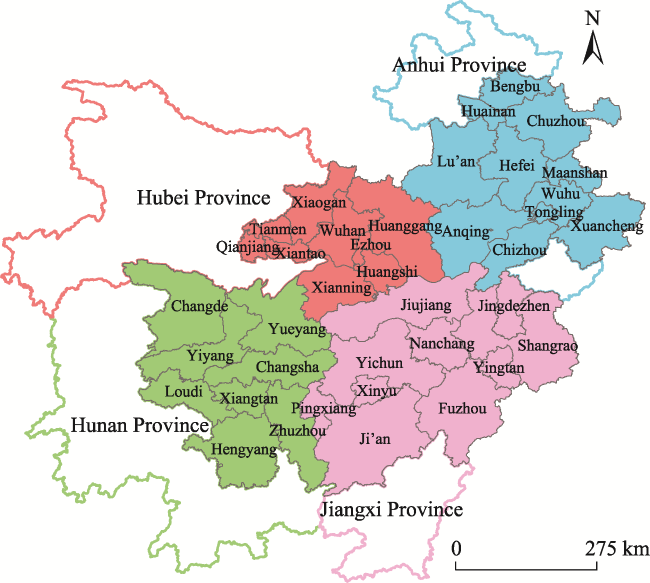
Fig. 1 Location and spatial organization of the four-city area in central China
There are numerous rivers and densely covered lakes in the four-city area in central China, and these are the regions with the most abundant water resources in China. However, with the continuous increase in regional urbanization, rapid economic development, and the substantial increase in regional GDP, the urban social economy and water ecological environmental problems have become increasingly prominent, as exemplified by heavy river basin pollution, frequent seasonal water quality deficiencies and water shortages, shrinking lakes, drying wetlands, excessive water use, and serious waste issues. Therefore, in the present study, we perform a coordinated analysis of the regional water resource utilization and regional socioeconomic factors associated with urbanization in urban agglomerations.

2.2 Methods

2.2.1 Super-SBM-DEA model

In this study, a super-SBM-DEA model with unexpected output is applied to assess GWRUE in four-city area in central China. Here, a production system with n DMUs is structured, and each unit has three factors: inputs, expectedoutput and unexpected output, as represented by the three vectors xRm, ygRs1, and ybRs2, where m, s1 and s2 are the numbers of inputs, expected output and unexpected output, respectively. The matrices X, Yg, and Yb are defined as follows:
$\begin{align} & X=\left[ {{x}_{1}},{{x}_{2}},\ldots,{{x}_{n}} \right]\in {{R}^{m\times n}}, \\ & {{Y}^{g}}=\left[ y_{1}^{g},y_{2}^{g},\ldots,y_{n}^{g} \right]\in {{R}^{{{s}_{1}}\times n}}, \\ & {{Y}^{b}}=\left[ y_{1}^{b},y_{2}^{b},\ldots,y_{n}^{b} \right]\in {{R}^{{{s}_{2}}\times n}} \\ \end{align}$
Assuming that X > 0, Yg > 0, and Yb > 0, then the production possibility set (P) can be defined as:
$P=\left\{ \left( x,{{y}^{g}},{{y}^{b}} \right)\text{ }\!\!|\!\!\text{ }x\ge X\lambda,{{Y}^{g}}\le {{Y}^{g}}\lambda,{{Y}^{b}}\ge {{Y}^{b}}\lambda,\lambda \ge 0 \right\}$
where λ is a nonnegative vector of weights assigned to inputs and outputs. The three inequalities in the P function represent the situation when the actual input level is greater than the frontier investment level, the actual expected output level is lower than the frontier expected output level, and the actual unexpected output is greater than the leading edge of the unexpected output level (Li et al., 2013). According to Tone’s theoretical model (Tone, 2004), the SBM model dealing with unexpected output for evaluating DMU (x0, yg 0, yb 0) is as follows:
$\begin{align} & \left[ Unexpected outputs\ SBM \right]\rho = \\ & min\frac{1-\frac{1}{m}\sum\limits_{i=1}^{m}{\frac{S_{i}^{-}}{{{x}_{i0}}}}}{1+\frac{1}{{{s}_{1}}+{{s}_{2}}}\left( \sum\limits_{r=1}^{{{s}_{1}}}{\frac{S_{r}^{g}}{y_{r0}^{g}}+\sum\limits_{r=1}^{{{s}_{2}}}{\frac{S_{r}^{b}}{y_{r0}^{b}}}} \right)} \\ \end{align}$
$~Subject to \left\{ \begin{align} & {{x}_{i0}}=\underset{j=1}{\overset{n}{\mathop{\mathop{\sum }^{}}}}\,{{x}_{ij}}{{\lambda }_{j}}+S_{i}^{-}\text{ }\left( i=1,2,\cdots,m \right) \\ & y_{r0}^{g}=\underset{j=1}{\overset{n}{\mathop{\mathop{\sum }^{}}}}\,y_{rj}^{g}{{\lambda }_{j}}-S_{r}^{g}\text{ }\left( r=1,2,\cdots,{{s}_{1}} \right) \\ & y_{r0}^{b}=\underset{j=1}{\overset{n}{\mathop{\mathop{\sum }^{}}}}\,y_{lj}^{b}{{\lambda }_{j}}+S_{l}^{b}\text{ }\left( l=1,2,\cdots,{{s}_{2}} \right) \\ & S_{i}^{-}>0,S_{r}^{g}>0,S_{l}^{b}>0,{{\lambda }_{j}}>0,\mathop{\sum }^{}{{\lambda }_{j}}=1 \\ \end{align} \right.$
where S-, Sg and Sb denote slack vectors corresponding to the excess of inputs, shortage of expected output and excess of unexpected output, respectively. The target function value of ρ is the efficiency value of the DMU, taking values in the range [0,1]. When ρ = 1 and S- = Sg = Sb = 0, the estimated DMU is SBM-efficient. When ρ < 1, the DMU is inefficient. In addition, there may be more than one SBM-efficient DMU when multiple units have efficiency values equal to 1. Therefore, appropriate adjustments must be made for the inputs and outputs in such units. To further rank these DMUs and provide more accurate efficiency evaluation values, on the basis of the SBM model and combined with the research of Tone (2002) and Li et al. (2013), this paper gives the super-SBM-DEA model with unexpected outputs, which is applied to evaluate SBM-efficient DMUs. The model is written as follows (Tone, 2003):
$\begin{align} & \left[ \mathrm{Unexpected o}utputs\ Super\ SBM \right]{{\rho }^{*}}= \\ & min\frac{\frac{1}{m}\sum\limits_{i=1}^{m}{\frac{{\bar{x}}}{{{x}_{i0}}}}}{\frac{1}{{{s}_{1}}+{{s}_{2}}}\left( \sum\limits_{r=1}^{{{s}_{1}}}{\frac{{{{\bar{y}}}^{g}}}{y_{r0}^{g}}}+\sum\limits_{r=1}^{{{s}_{2}}}{\frac{{{{\bar{y}}}^{b}}}{y_{r0}^{b}}} \right)} \\ \end{align}$
$~Subject to \left\{ \begin{align} & \text{ }\bar{x}=\underset{j=1,\text{ j}\ne {{j}_{0}}}{\overset{n}{\mathop{\mathop{\sum }^{}}}}\,{{x}_{ij}}{{\lambda }_{j}}\text{ }\left( i=1,2,\cdots,m \right) \\ & \text{ }{{{\bar{y}}}^{g}}=\underset{j=1,\text{ j}\ne {{j}_{0}}}{\overset{n}{\mathop{\mathop{\sum }^{}}}}\,y_{rj}^{g}{{\lambda }_{j}}\text{ }\left( r=1,2,\cdots,{{s}_{1}} \right) \\ & \text{ }{{{\bar{y}}}^{b}}=\underset{j=1,\text{ j}\ne {{j}_{0}}}{\overset{n}{\mathop{\mathop{\sum }^{}}}}\,y_{lj}^{b}{{\lambda }_{j}}\text{ }\left( l=1,2,\cdots,{{s}_{2}} \right) \\ & \text{ }\bar{x}\ge {{x}_{ij}},{{{\bar{y}}}^{g}}\le y_{rj}^{g},{{{\bar{y}}}^{b}}\ge y_{lj}^{b},{{\lambda }_{j}}>0 \\ \end{align} \right.$
where ρ* denotes the target function, and its efficiency value can be larger than 1, while other variables have similar implications as in Eq. (1). $\bar{x}$, ${{\bar{y}}^{g}}$, and ${{\bar{y}}^{b}}$ are the mean vector of the input vector, expected output vector and unexpected output vector, respectively. As the models discussed above are all under the assumption of constant returns to scale, we can also relax and extend these models to the variable returns-to-scale condition with the restrictions $\underset{i=1}{\overset{n}{\mathop \sum }}\,{{\lambda }_{i}}=1$ in Eq. (3) and $\sum\limits_{i=1,\text{ i}\ne {{i}_{0}}}^{n}{{{\lambda }_{i}}=1}$ in Eq. (4). Thus, a super-SBM DEA model is developed to evaluate the GWRUE of the four cities in central China in this study.

2.2.2 Standard deviational ellipse

The standard deviational ellipse (SDE) is one of the classical spatial statistical methods (Lefever, 1926) and can accurately reveal the spatial distribution characteristics and evolution of geographical elements by calculating the parameters of centrality, coordinates, azimuth, major axis and minor axis, area, oblateness, etc. It has been widely used to quantitatively describe the spatial distribution characteristics and spatiotemporal evolution of social and economic elements (Muhammad et al., 2019; Tian et al., 2019; Lu et al., 2020; Huang et al., 2021) and natural geographical elements (Han et al., 2020; Yuan et al., 2020; Chen et al., 2021). The parameters of SDE are calculated as follows (Du et al., 2019; Yuan et al., 2020; Chen et al., 2021):
(1) Plane gravity center and moving parameters
$X=\underset{j=1}{\overset{n}{\mathop \sum }}\,{{w}_{j}}{{x}_{j}}/\underset{j=1}{\overset{n}{\mathop \sum }}\,{{w}_{j}};\ \ Y=\underset{j=1}{\overset{n}{\mathop \sum }}\,{{w}_{j}}{{y}_{j}}/\underset{j=1}{\overset{n}{\mathop \sum }}\,{{w}_{j}}$
where wj represents the weight value of the GWRUE of region j and xj and yj represent the longitude and latitude coordinates of region j, respectively. X and Y represent the longitude and latitude coordinates of the gravity center, respectively, whose changes over time can reflect the evolutionary route and relative position of GWRUE spatial variation patterns.
${{D}_{ab}}=C\times \sqrt{{{({{X}_{a}}-{{X}_{b}})}^{2}}+{{({{Y}_{a}}-{{Y}_{b}})}^{2}}}$
${{V}_{ab}}=\sqrt{{{({{X}_{b}}-{{X}_{a}})}^{2}}+{{({{Y}_{b}}-{{Y}_{a}})}^{2}}}/(b-a)$
$\begin{align} & {{\theta }_{ab}}= \\ & \left\{ \begin{array}{*{35}{l}} \text{ }degrees\left\{ arctan\left[ ({{Y}_{a}}-{{Y}_{b}})/({{X}_{a}}-{{X}_{b}}) \right] \right\},\ \ \ \ \ \ \text{ }{{X}_{a}}>{{X}_{b}},\ {{Y}_{a}}\ne {{Y}_{b}} \\ ~degrees\left\{ arctan\left[ ({{Y}_{a}}-{{Y}_{b}})/({{X}_{a}}-{{X}_{b}}) \right]+\pi \right\},\text{ }{{X}_{a}}<{{X}_{b}},\ {{Y}_{a}}>{{Y}_{b}} \\ ~degrees\left\{ arctan\left[ ({{Y}_{a}}-{{Y}_{b}})/({{X}_{a}}-{{X}_{b}}) \right]-\pi \right\},\text{ }{{X}_{a}}<{{X}_{b}},\ {{Y}_{a}}<{{Y}_{b}} \\ \ {{0}^{\circ }},\ \text{ }\ \ \ \ \ \ \ \ \ \ \ \ \ \ \ \ \ \ \ \ \ \ \ \ \ \ \ \ \ \ \ \ \ \ \ \ \ \ \ \ \ \ \ \ \ \ \ \ \ \ \ \ \text{ }{{X}_{a}}>{{X}_{b}},\ {{Y}_{a}}={{Y}_{b}} \\ \ \pm {{180}^{\circ }},\ \ \ \ \ \ \ \ \ \ \ \ \ \ \ \ \ \ \ \ \ \ \ \ \ \ \ \ \ \ \ \ \ \ \ \ \ \ \ \ \ \ \ \ \ \ \ \ \ \text{ }{{X}_{a}}<{{X}_{b}},\ {{Y}_{a}}={{Y}_{b}} \\ \text{ }{{90}^{\circ }},\ \ \ \ \ \ \ \ \ \ \ \ \ \ \ \ \ \ \ \ \ \ \ \ \ \ \ \ \ \ \ \ \ \ \ \ \ \ \ \ \ \ \ \ \ \ \ \ \ \ \ \ \text{ }{{X}_{a}}={{X}_{b}},\ {{Y}_{a}}>{{Y}_{b}} \\ \text{ }-{{90}^{\circ }},\ \ \ \ \ \ \ \ \ \ \ \ \ \ \ \ \ \ \ \ \ \ \ \ \ \ \ \ \ \ \ \ \ \ \ \ \ \ \ \ \ \ \ \ \ \ \ \ \ \text{ }{{X}_{a}}={{X}_{b}},\ {{Y}_{a}}<{{Y}_{b}} \\\end{array} \right. \\ \end{align}$
where Dab refers to the moving distance of the gravity center from year a to year b in km; C represents the coefficient of the geographical coordinates of the plane distance, which equals 111.111 km. Vab denotes the moving speed of the gravity center (km/yr). θab denotes the angle of the gravity center, degrees {} turns radians into angles, and θ denotes the shifted angle of the gravity center between different years (-180° ≤ θ ≤ 180°), which specifically represents the shifted direction. Specifically, the angle of the due east direction is 0°, counterclockwise rotation is positive, and clockwise rotation is negative. If 0° < θ < 90°, it implies that the gravity center shifts to the northeast; if 90° < θ < 180°, it implies that the gravity center shifts to the northwest; if -90° < θ < 0°, it implies that the gravity center shifts to the southeast; if -180° < θ < -90°, it implies that the gravity center shifts to the southwest; if θ is ±180°, it implies that the gravity center shifts to due west; if θ is 90°, it implies that the gravity center shifts to due north or due south (Hu et al., 2020).
(2) Azimuth angle
The azimuth angle formula is as follow:
$\tan \theta_{a b}^{\prime}=\frac{\left(\sum_{j=1}^{n} w_{j}^{2} x_{j}^{\prime 2}-\sum_{j=1}^{n} w_{j}^{2} y_{j}^{\prime 2}\right)+\sqrt{\left(\sum_{j=1}^{n} w_{j}^{2} x_{j}^{\prime 2}-\sum_{j=1}^{n} w_{j}^{2} y_{j}^{\prime 2}\right)^{2}+4 \sum_{j=1}^{n} w_{j}^{2} x_{j}^{\prime 2} y_{j}^{\prime 2}}}{2 \sum_{j=1}^{n} w_{j}^{2} x_{j}^{\prime} y_{j}^{\prime}}$
where $\theta_{a b}^{\prime}$ denotes the angle movement of the gravity center from year a to year b; if $\theta_{a b}^{\prime}=0$, then it represents the east position. The angle is clearly defined, which demonstrates the main orientation of the geographical units (Gong, 2010). The azimuth reflects the main trend direction of GWRUE spatial variation patterns.
(3) Major axis and minor axis
The major axis and minor axis formulas are as follows:
$\begin{array}{c} \sigma_{x}=\sqrt{\frac{\sum_{j=1}^{n}\left(w_{j} x_{j}^{\prime} \cos \theta-w_{j} y_{j}^{\prime} \sin \theta\right)^{2}}{\sum_{j=1}^{n} w_{j}^{2}}} \\ \sigma_{y}=\sqrt{\frac{\sum_{j=1}^{n}\left(w_{j} x_{j}^{\prime} \sin \theta-w_{j} y_{j}^{\prime} \cos \theta\right)^{2}}{\sum_{j=1}^{n} w_{j}^{2}}} \end{array}$
where σx and σy denote the major axis and minor axis, respectively, which indicate the directions and scope of GWRUE spatial variation and the dispersion degree among different regions.
(4) Area and oblateness of the ellipse
The area and oblateness of the ellipse formulas are as follows:
$S=\pi {{\sigma }_{x}}{{\sigma }_{y}};\ \ \varphi =\frac{{{\sigma }_{x}}-{{\sigma }_{y}}}{{{\sigma }_{x}}}$
where S and φ denote the area and oblateness of the ellipse, respectively. The area size of the ellipse represents the degree of concentration (dispersion) for GWRUE spatial variation. The oblateness value of the ellipse is between 0 and 1, which reflects the orientation of GWRUE spatial variation. The larger the gap and the greater the ratio is between the two, the greater the distribution, and the longer the shape is, the more directional.

2.2.3 Geographical detector model

The geographical detector model (GDM) was proposed by Wang et al. (2020) based on spatial variance analysis, which is a novel statistical method used to reveal the driving factors of the spatial variation of geographical elements. This method has been widely applied to quantify the influence of potential driving factors on geospatial elements (Wu et al., 2016; Zhou et al., 2018a; Bai, 2019; Luo et al., 2019; Wei et al., 2020; Fang et al., 2021; Song and Wu, 2021). The geographical detector model consists of four modules, namely, factor detector, interaction detector, risk detector and ecological detector. In this study, factor detection and interaction detection are adopted to examine the explanatory powers of different influencing factors for the spatiotemporal variation in GWRUE in the four-city area in central China.
Factor detection is used to identify the spatial differentiation of dependent variable Y (GWRUE value) and the explanatory power of independent variable X on the spatial differentiation of the Y value. It is calculated according to the following q-statistic (Wei et al., 2020; Gao et al., 2021):
$q=1-\frac{\sum\limits_{k=1}^{M}{{{N}_{k}}\mu _{k}^{2}}}{N{{\mu }^{2}}}=1-\frac{SSW}{SST}$
$SSW=\underset{k=1}{\overset{M}{\mathop \sum }}\,{{N}_{k}}\mu _{k}^{2},\ \ \ \ SST=N{{\mu }^{2}}$
where q is the explanatory power of influencing factors for the spatial differentiation of GWRUE, and its value lies between zero and one. The larger the value is, the stronger the explanatory power of these influencing factors on the spatial differentiation of GWRUE. k is the number of strata for variable Y or X. N refers to the total number of spatial units over the entire study area, Nk represents the number of units in strata k. μ2 and μ2 k denote the global variance of the dependent variable in the entire study area and the variance of the dependent variable in strata k, respectively. SSW and SST denote the within sum of squares and total sum of squares, respectively.
An interaction detector can also be applied to identify the interaction between any two factors (symbolized by ∩). The influence of two influencing factors on the spatiotemporal variation in GWRUE may be independent or dependent, and the influence on the spatiotemporal variation in GWRUE may be stronger or weaker after interaction. Their interaction relationships are identified by comparing the interaction q value of the two factors and the q value of each of the two factors (Wang et al., 2010), and the specific relationship categories are summarized as follows:
Independent: q(X1X2) = q(X1) + q(X2)
Univariate weakening: Min(q(X1), q(X2)) < q(X1X2) < Max(q(X1), q(X2))
Nonlinear weakening: q(X1X2) < min(q(X1), q(X2))
Nonlinear enhancement: q(X1X2) > q(X1) + q(X2)
Bivariate enhancement: Max (q(X1), q(X2)) < q(X1X2) < q(X1) + q(X2)

2.3 Variable selection and data source

2.3.1 Input and output variable

In the literature on water use efficiency, it is generally considered that the most important input elements are capital, labor and water resources. In this study, based on existing studies (Deng et al., 2016; Wang et al., 2018; Hu and Jiao, 2019; Zhang et al., 2020a), capital investment, labor, and the water resource ecological footprint (WREF) are selected as input elements. Gross domestic product (GDP) and Human Sustainable Development Index (HSDI) are employed as expected outputs, and the water pollution ecological footprint (WPEF) is selected as the unexpected output. The specific variables are explained below.
(1) Capital investment
The fixed assets investment of the whole society over the years is used as capital input (Chen and Jia, 2017; Zhou et al., 2018b; Yu et al., 2019), and the total fixed assets investment over the years was converted into 2000 prices (constant prices) using the fixed asset investment price index.
(2) Labor force
The number of employed persons at each year’s end in different regions is selected to represent actual labor input.
(3) WREF
The water resources ecological footprint (i.e., water volume ecological footprint) refers to water resource consumption by human beings for production and life (Wang and Liu, 2019), and the total water resource ecological footprint in the region was selected as the water resource input, excluding the water quality ecological footprint. The water resource ecological footprint in the region was calculated by using the research method of Li et al. (2020). Due to space limitations, the detailed calculation method is not repeated here.
(4) GDP
The GDP of each region in the four-city area in central China is adopted as the expected output, and the GDP over the years is converted into 2000 prices (constant prices) using the producer’s price index.
(5) HSDI
The Human Sustainable Development Index (HSDI) adds an environmental dimension to the Human Development Index (HDI), which already covers two of the three dimensions of sustainability, namely, the social and economic dimensions (Goodland, 1995), to build a true human sustainable development index (Togtokh, 2011). In this paper, the HSDI adds an environmental dimension to the HDI, namely, per capita industrial wastewater discharge, per capita industrial waste gas discharge, per capita industrial solid waste emissions and per capita electricity consumption. The HSDI is calculated and transformed to obtain the environmental performance index, which is implanted into the income index and modified to obtain the HSDI (Tian et al., 2007) containing environmental impact factors, which is taken as the expected output. Each of these indicators is indexed within a range defined by maximum and minimum values. The specific calculation formula (Bravo, 2014, 2015; Wang, 2016; Hickel, 2020) is as follows:
${{H}_{1}}=\frac{ELB-25}{85-25}$
${{H}_{2}}=\left( \frac{AL}{100} \right)\times \frac{2}{3}+\left( \frac{ER}{100} \right)\times \frac{1}{3},\ \ ER=\frac{{{P}_{primary}}+{{P}_{high}}+{{P}_{college}}}{Po{{p}_{\left( 6-22\text{ }yr \right)}}}$
$\begin{align} & {{H}_{3}}=\frac{\ln GDP-ln100}{\ln 40000-ln100}~ \\ & {{H}_{3}}P={{\left[ \frac{1}{2}{{\left( {{H}_{3}} \right)}^{1-\varepsilon }}+\frac{1}{2}{{\left( 1-PI \right)}^{1-\varepsilon }} \right]}^{\frac{1}{1-\varepsilon }}} \\ \end{align}$
$HSDI=\frac{{{H}_{1}}+{{H}_{2}}+{{H}_{3}}P}{3}~$
where HSDI is the Human Sustainable Development Index. H1 denotes life expectancy, and ELB is the average life expectancy in each region (unit: year). H2 is the educational development index, where AL is the adult literacy rate (%), ER is the comprehensive gross enrollment ratio at all levels of education, Pprimary is the number of enrolled primary school students, Phigh is the number of enrolled middle school students (junior high school and senior high school), Pcollege is the number of students in college, and Pop(6-22 yr) is the school-age population aged 6-22 years in each region. H3P is environmental impact index. H3 is the GDP index. PI is the comprehensive environmental loss index, which is determined by the arithmetic mean of the four indexes of per capita industrial wastewater discharge, per capita industrial waste gas discharge, per capita industrial solid waste emissions and per capita electricity consumption, namely, PI = (PI1+PI2+PI3+PI4). According to the data collection and trend analysis over the years, 200 t person-1, 400000 standard m3 person-1, 0.3 t person-1, and 15000 kWh person-1 are selected as the maximum values of per capita wastewater discharge, per capita waste gas emissions, per capita industrial solid waste emissions, and per capita electricity consumption, respectively, and their minimum value is 0. Therefore, through PI1 = per capita industrial wastewater discharge, PI2 = per capita industrial waste gas discharge/400000, PI3 = per capita industrial solid waste discharge/0.3 and PI4 = per capita electricity consumption/15000, the four environmental resource indicators are standardized into corresponding environmental resource loss indexes (PI1PI2PI3 and PI4). According to the correction method proposed by Atkinson (1970), the ε value in this paper is 2 for the data operation of the HSDI.
(6) WPEF
The water pollution ecological footprint (i.e., water quality ecological footprint) refers to the area of water resources needed to absorb pollutants produced by a certain population that exceed the carrying capacity of the existing water body and to dilute the pollutants to a certain water quality standard (Wang and Liu, 2019). In this article focused on the four-city area in central China, total emission reduction indicators for major pollutants—chemical requirements (COD) and ammonia nitrogen (NH) emissions—are selected as the research content and unexpected output. Because the two pollutants have obvious overlap in environmental impacts, the largest pollution footprint among them is taken as the final water pollution ecological footprint. The water pollution ecological footprint in the region is calculated by using the research method of Feng and Zhao (2020). Due to space limitations, the detailed calculation method is not repeated here.

2.3.2 Influencing factors of GWRUE

To better explain the formation mechanism of the spatiotemporal differentiations of GWRUE in the four-city area in central China, it is necessary to conduct empirical tests on the influencing factors. However, there are many factors affecting GWRUE (Deng et al., 2016). Therefore, based on the existing literature (Deng et al., 2016; Fang et al., 2017; Wang et al., 2018; Zhou et al., 2018a; Ding et al., 2019a; Hu and Jiao, 2019; Zhang et al., 2019; Zhang et al., 2020a) and the principles of data accessibility, observability and representativeness, this paper finally takes GWRUE as the dependent variable and selects the influencing factors of GWRUE spatiotemporal differentiation as the independent variables. The factors influencing GWRUE are selected as shown in Table 1.
Table 1 Explanations of influencing factors of the GWRUE in the four-city area in central China
Influencing factors Implication Abbreviation Unit
Water resource abundance (X1) Per capita water supply WRA m3 person-1
Population density (X2) The resident population per square kilometer PD person km-2
Economic development level (X3) The proportion of the GDP to the local population EDL yuan person-1
Medical resource possession (X4) The number of practicing (or assistant) physicians MRP person
Proportion of agriculture water use (X5) The proportion of agricultural water consumption to regional total water consumption PAWU %
Proportion of industrial water use (X6) The proportion of industrial water consumption to regional total water consumption PIWU %
Proportion of domestic water use (X7) The proportion of domestic water consumption to regional total water consumption PDWU %
Foreign trade dependence (X8) The proportion of import and export trade value to GDP FTD %
Industrial transformation degree (X9) The proportion of tertiary industry value added to GDP ITD %
Science and education level (X10) The proportion of science and education expenditure to local financial expenditure SEL %
Dependence degree of foreign actual investment (X11) The proportion of foreign direct investment to GDP DDFAI %
Urban dependence on real estate (X12) The proportion of total investment in real estate development to GDP UDRE %

2.3.3 Data sources

Based on data availability, the scope of the study included the administrative regions of each city. Each indicator data point was derived from the Statistical Yearbooks (2011- 2020) of Hubei Province, Hunan Province, Jiangxi Province and Anhui Province, as well as the Water Resources Bulletin of Each Province (2011-2020), the Statistical Yearbook, Statistical Bulletin on National Economic and Social Development and Statistical Bulletin of the Environmental Situation of 38 Cities in the Four-city Area in Central China from 2011 to 2020. The missing data are supplemented according to the environmental protection planning of provinces and prefecture-level cities.

3 Results and analysis

3.1 GWRUE measurement in the four-city area in central China

As shown in Table 2, during the study period, the overall level of GWRUE in the four-city area in central China was low, and the variation among regions was large. In addition, the change in GWRUE in most regions decreased over time. This showed that there is still much room for improvement in GWRUE in the four-city area in central China. This result is also consistent with the results of Zhang et al. (2020a) in their study of the dynamic evaluation of water resource green efficiency in China. During 2010-2019, the highest annual GWRUE in the four-city area in central China was in 2010, while the lowest was in 2019. In addition, the region with the highest GWRUE was Qianjiang and the lowest in Shangrao (Table 2).
Table 2 GWRUE in the four-city area in central China during 2010-2019
Region 2010 2011 2012 2013 2014 2015 2016 2017 2018 2019 Average
Wuhan 1.101 1.044 1.057 1.069 1.082 1.068 1.089 1.084 1.047 0.219 0.986
Huangshi 0.663 0.697 0.694 0.646 0.625 0.568 0.564 0.588 0.572 2.404 0.802
Ezhou 0.792 0.841 0.832 1.032 1.036 1.025 0.791 1.186 0.782 1.001 0.932
Xiaogan 0.442 0.398 0.391 0.371 0.392 0.395 0.393 0.380 0.377 0.188 0.373
Huanggang 0.340 0.326 0.325 0.308 0.322 0.341 0.354 0.346 0.333 0.154 0.315
Xianning 0.488 0.475 0.475 0.484 0.497 0.489 0.523 0.455 0.500 0.297 0.468
Xiantao 1.015 1.000 1.002 1.004 1.003 1.012 1.002 0.763 0.744 0.508 0.905
Qianjiang 1.095 1.187 1.153 1.147 1.145 1.093 1.111 1.169 1.136 1.056 1.129
Tianmen 1.035 1.034 1.032 1.039 1.039 1.040 1.031 0.732 1.029 1.055 1.007
Changsha 1.002 1.031 1.025 1.034 1.027 1.017 1.001 1.006 1.032 0.215 0.939
Zhuzhou 0.594 0.573 0.583 0.488 0.514 0.593 0.551 0.544 0.536 1.397 0.637
Xiangtan 0.581 0.575 0.566 0.521 0.551 0.574 0.547 0.552 0.566 0.249 0.528
Hengyang 0.709 0.432 1.013 0.337 0.361 0.405 0.388 0.372 0.347 0.181 0.454
Changde 1.074 1.068 1.042 1.035 1.037 1.054 1.009 0.547 0.555 0.221 0.864
Yueyang 0.704 0.503 1.012 0.607 0.615 0.558 0.478 0.379 0.380 0.195 0.543
Yiyang 0.557 0.449 0.464 0.428 0.453 0.477 0.446 0.436 0.447 0.206 0.436
Loudi 0.740 0.528 0.530 0.489 0.510 0.541 0.512 0.502 0.500 0.235 0.509
Nanchang 1.025 0.514 0.527 0.510 0.517 0.517 0.498 0.614 0.610 0.209 0.554
Jingdezhen 0.773 0.737 0.780 0.729 0.751 0.788 0.804 0.719 0.653 0.512 0.724
Pingxiang 0.701 0.712 1.000 0.650 0.695 1.024 1.023 1.020 1.010 0.574 0.841
Jiujiang 0.454 0.367 0.394 0.381 0.405 0.442 0.422 0.444 0.470 0.223 0.400
Xinyu 1.128 1.032 1.060 1.055 1.048 1.088 1.144 1.059 1.142 1.014 1.077
Yingtan 1.070 0.838 1.022 0.850 0.881 0.916 1.064 1.054 1.044 1.045 0.978
Ji’an 0.338 0.312 0.323 0.328 0.346 0.371 0.349 0.340 0.346 0.170 0.322
Yichun 0.388 0.313 0.368 0.308 0.321 0.341 0.344 0.371 0.354 0.179 0.329
Fuzhou 0.406 0.382 0.407 0.397 0.417 0.430 0.429 0.429 0.415 0.197 0.391
Shangrao 0.331 0.302 0.330 0.301 0.320 0.341 0.339 0.342 0.332 0.167 0.310
Hefei 1.149 1.048 0.605 0.674 0.723 1.011 1.114 1.109 1.070 0.218 0.872
Wuhu 0.611 0.522 0.532 0.584 0.588 0.590 0.523 0.575 0.535 0.241 0.530
Bengbu 0.506 0.563 0.566 0.493 0.552 0.623 0.505 0.511 0.471 0.247 0.504
Huainan 0.602 0.551 0.586 0.489 0.516 0.492 0.428 0.435 0.403 0.223 0.473
Maanshan 0.553 0.609 0.547 0.614 0.614 0.523 0.514 0.575 0.535 0.303 0.539
Tongling 1.253 1.369 1.395 1.110 1.093 1.047 0.556 0.596 0.562 0.230 0.921
Anqing 0.406 0.450 0.490 0.424 0.455 0.423 0.461 0.414 0.391 0.343 0.426
Chuzhou 0.384 0.370 0.372 0.366 0.408 0.411 0.372 0.370 0.349 0.217 0.362
Lu’an 0.426 0.319 0.333 0.319 0.332 0.356 0.399 0.381 0.342 0.179 0.339
Chizhou 0.627 1.015 1.018 1.105 1.033 1.087 0.701 0.499 1.025 0.400 0.851
Xuancheng 0.433 0.528 0.553 0.547 0.554 0.533 0.500 0.504 0.464 0.268 0.488
Average 0.697 0.658 0.695 0.639 0.652 0.674 0.639 0.616 0.616 0.446 0.633
The GWRUE values in Qianjiang and Xinyu were all greater than 1 during 2010-2019 (Table 2), meaning that the GWRUE of these two regions improved. However, the GWRUE value of most regions was less than 1 during the study period; that is, the GWRUE of these regions deteriorated. In addition, according to mean efficiencies, these regions did not achieve an effective input and output of green water resources. For example, there were 22 regions with average GWRUE values less than 0.6. Therefore, the input-output ratio must be adjusted to improve the GWRUE based on high-quality economic development. This result is similar to the results of Wang et al. (2018) in their study of water use efficiency in 30 provinces of China.
Most regions had relatively unstable efficiency across time periods. For example, Chizhou presented significantly worse values in 2016, 2017 and 2019, Tianmen in 2017, Zhuzhou in 2016-2018, and Hengyang, Changde, Jingdezhen, Wuhu, Anqing, and Xuancheng in 2017-2019. Huangshi and Zhuzhou presented significantly better values in 2019, Pingxiang and Hefei in 2015-2018, and Yingtan in 2016-2019. These results indicated that these regions in the four-city area in central China must develop more stable and effective water management strategies and more active environmental protection mechanisms.

3.2 Spatiotemporal variations analysis of GWRUE

According to the GWRUE value, the ArcGIS SDE tool was used to obtain the relevant parameters of gravity centers—SDE and the spatial movement path (Fig. 2, Table 3 and Table 4)—and then the spatiotemporal variation characteristics of GWRUE in the four-city area in central China were analyzed by the relevant parameters of SDE.
Fig. 2 Standard deviational ellipse and gravity center movement path of GWRUE in the four-city area in central China
Table 3 Gravity center moving direction and distance of SDEs for GWRUE in the four-city area in central China from 2010 to 2019
Year Gravity center coordinates Moving angle (°) Moving direction Moving distance (km) Moving speed
(km yr-1)
2010 115.06°E, 29.76°N - - - -
2011 115.09°E, 29.79°N 57.57 Northeast 3.93 3.69
2012 114.98°E, 29.63°N -114.41 Southwest 21.24 20.36
2013 115.01°E, 29.67°N 66.43 Northeast 5.93 5.70
2014 115.06°E, 29.76°N 66.46 Northeast 11.56 11.10
2015 115.06°E, 29.72°N -87.65 Southeast 4.14 4.13
2016 114.99°E, 29.67°N -130.26 Southwest 9.80 9.05
2017 115.10°E, 29.68°N 13.33 Northeast 12.04 10.51
2018 115.09°E, 29.66°N -111.07 Southwest 2.56 2.48
2019 114.92°E, 29.50°N -124.49 Southwest 25.30 23.72
Table 4 SDE parameters of the spatial variation pattern of GWRUE in the four-city area in central China during 2010-2019
Year Ellipse area (km2) Ellipse
azimuth θ ° (°)
Ellipse
oblateness
Major axis (km) Minor axis (km)
2010 191798.29 48.92 0.41 643.38 379.59
2011 195345.20 47.38 0.43 658.57 377.70
2012 197234.11 46.00 0.42 660.63 380.16
2013 197429.25 46.05 0.42 656.98 382.65
2014 193717.96 48.05 0.41 647.00 381.25
2015 195817.68 46.26 0.41 651.72 382.59
2016 196611.43 46.01 0.39 639.53 391.46
2017 192831.61 43.44 0.40 639.13 384.17
2018 192874.26 44.64 0.39 635.54 386.43
2019 172170.15 41.26 0.31 561.79 390.23

3.2.1 Analysis of the spatial movement path of SDE gravity centers

As shown in Fig. 2 and Table 3, the gravity centers at each characteristic time point of GWRUE in the four-city area in central China were between 114.92°E-115.10°E and 29.50°N-29.79°N. In 2010, the coordinates of the SDE gravity centers were (115.06°E, 29.76°N), located in Huangshi City, Hubei Province. Then, by 2019, the coordinates of the SDE gravity center were 114.92°E, 29.50°N, located in Xianning City, Hubei Province. From 2010 to 2013, the spatial movement path of the SDE gravity centers experienced an overall shift from northeast (2011) to southwest (2012) to northeast (2013), with an average annual moving distance of 10.37 km and an average annual moving speed of 9.92 km yr-1. Among them, the maximum moving distance and speed in 2012 were 21.24 km and 20.36 km yr-1, respectively. From 2014 to 2016, the spatial movement path of SDE gravity centers experienced an overall shift from northeast (2014) to southeast (2015) to southwest (2016), with an average annual moving distance of 8.50 km and an average annual moving speed of 8.09 km yr-1. Among them, the maximum moving distance and speed in 2014 were 11.56 km and 11.01 km yr-1, respectively. From 2017 to 2019, the spatial movement path of the SDE gravity centers experienced an overall shift from northeast (2017) to southwest (2018 and 2019), with an average annual moving distance of 13.30 km and an average annual moving speed of 12.24 km yr-1. Among them, the maximum moving distance and speed in 2019 were 23.30 km and 23.72 km yr-1, respectively. In brief, during the study period, the moving speed of the SDE gravity centers for GWRUE in the four- city area in central China showed a “waveform” rising trend.

3.2.2 Main parameters of SDE

As shown in Table 4, during the study period, the SDE range of each characteristic time point showed a decreasing trend, indicating that the spatial variation pattern of GWRUE in the four-city area in central China tended to be agglomerated. On the whole, the ellipse area showed a trend of increasing-decreasing-increasing-decreasing, which implied that during the study period, the spatial variation patterns of GWRUE in the four-city area in central China showed an annual change trend of dispersion-agglomeration- decentralization-agglomeration. Ellipse oblateness decreased from 0.41 in 2010 to 0.31 in 2019, indicating that the direction of the spatial variation pattern of GWRUE became weaker. From 2010 to 2019, the spatial variation pattern of GWRUE was north to south (Fig. 2 and Table 3), and the azimuth decreased by 7.66° (Table 4). The shift trend of the spatial variation pattern was obvious, which indicated that the spatial variation pattern of GWRUE in the four-city area in central China changed from northeast to southwest.
During the study period, the GWRUE of the four-city area in central China had a decreasing trend along the major axis in general, while the ellipse along the minor axis showed an increasing trend, which indicates that GWRUE tended to agglomerate along the major axis. The major axis decreased from 643.38 km in 2010 to 561.79 km in 2019, which meant that the GWRUE of the four-city area in central China was increasingly agglomerated in the main direction, and it was agglomerated in the southwest. That is, the GWRUE in the southwest was higher than that in the northeast. This was consistent with the recent trend of fast in the economic development in the southwest and slow development in the northeast in the four-city area in central China. The minor axis increased from 379.59 km in 2010 to 390.23 km in 2019, which meant that the spatial agglomeration degree of GWRUE in the east-south to west-north direction showed a downward trend; that is, the gap of GWRUE in the east and west of the four-city area in central China decreased.

3.3 Influencing factor analysis of GWRUE spatiotemporal variations

3.3.1 Dominant factor analysis

The q values measured by the geographical detector indicate the influence degree of each factor on the spatiotemporal variations in GWRUE. The larger a q value is, the stronger the influence of this factor on the spatial variations in GWRUE. As shown in Fig. 3, the influence of each factor on the spatial variations in GWRUE exhibits certain differences in different years.
Fig. 3 Factor detection results of GWRUE spatial variations in the four-city area in central China from 2010 to 2019
In 2010, the q values of 12 factors in ascending order were as follows: PDWU (0.034) < DDFAI (0.061) < WRA (0.086) < SEL (0.111) < UDRE (0.194) < ITD (0.237) < PD (0.253) < PAWU (0.257) < PIWU (0.265) < FTD (0.294) < MRP (0.306) < EDL (0.381). Among these factors, EDL, MRP and FTD were considered to be the main factors affecting the spatial variations in GWRUE. This finding issimilar to those of Dalin et al. (2014) and Ding et al. (2019a), who found that economic development level and foreign trade dependence can improve water use efficiency. Moreover, the research results from Wang et al. (2018) indicated that export dependence positively impacts water use efficiency. In addition, since urbanization continuously concentrates resources to improve efficiency and reap high benefits, the high-quality development of urbanization can not only promote the improvement in medical and health services in urban areas but also realize the improvement in water resource utilization efficiency (Guo, 2017). In 2013, by comparing the q values of 12 factors, MRP, EDL, and UDRE were considered to have the greatest influences on the spatial variations in GWRUE. Yang et al. (2017) also found that effective incentives and supervision mechanisms for real estate developers can promote the effective utilization of water resources. In 2016, the highest q values were found for EDL (0.369) and ITD (0.257), which indicated that EDL and ITD were the dominant factors causing the spatial variations in GWRUE. The research results from Shi et al. (2015) also showed that water use efficiency improves with the optimization of the industrial structure. In 2019, by comparing the q values of 12 factors, MRP and SEL were found to be the leading factors for the spatial variations in GWRUE. Previous studies demonstrated that investment in science, technology and education can be most conducive to water efficiency improvements (Colosimo and Kim, 2016; Wang et al., 2018; Wang et al., 2019; Wang et al., 2021).
By observing the changes in the influence of each factor, it can be found that the GWRUE was unchanged by the comprehensive effect of multiple factors, but on the whole, the influence of SEL and DDFAI gradually increased over time. Previous studies have shown that when socioeconomic development reaches a certain level, improving residents’ education levels and enhancing competencies in developing technological innovations and foreign direct investment agglomeration helps promote water use efficiency (Wang et al., 2018; Ding et al., 2019a).

3.3.2 Interaction analysis of influencing factors

As shown in Tables 5-8, the two-way interactions between different influencing factors showed an enhanced relationship, which was mainly manifested as a bivariate-enhanced relationship and a nonlinear-enhanced relationship and was especially affected by multiple factors that produced a nonlinear enhancement interaction. However, there is no weakening and independent relationship, which means that the effect of these factors on the spatiotemporal variations in GWRUE become greater after interaction.
Table 5 Interactive detection results of influencing factors for GWRUE spatial variations in the four-city area in central China in 2010
Factors WRA PD EDL MRP PAWU PIWU PDWU FTD ITD SEL DDFAI UDRE
WRA 0.086
PD 0.467↖ 0.253
EDL 0.478↗ 0.558↗ 0.381
MRP 0.413↗ 0.515↗ 0.700↗ 0.306
PAWU 0.478↖ 0.390↗ 0.483↗ 0.634↖ 0.257
PIWU 0.516↖ 0.384↗ 0.521↗ 0.570↗ 0.372↗ 0.265
PDWU 0.223↖ 0.298↗ 0.472↖ 0.426↖ 0.390↖ 0.457↖ 0.034
FTD 0.460↖ 0.551↗ 0.488↗ 0.506↗ 0.490↗ 0.482↗ 0.442↖ 0.294
ITD 0.479↖ 0.462↗ 0.517↗ 0.600↖ 0.465↗ 0.579↖ 0.445↖ 0.470↗ 0.237
SEL 0.430↖ 0.387↗ 0.562↖ 0.499↖ 0.457↖ 0.463↖ 0.433↖ 0.438↗ 0.486↖ 0.111
DDFAI 0.410↖ 0.457↖ 0.566↖ 0.589↖ 0.380↖ 0.412↖ 0.310↖ 0.451↖ 0.550↖ 0.364↖ 0.061
UDRE 0.431↖ 0.589↖ 0.623↖ 0.661↖ 0.523↖ 0.589↖ 0.570↖ 0.574↖ 0.492↖ 0.602↖ 0.692↖ 0.194

Note: ↘ represents a nonlinear weakening relationship; ↙ represents a univariate weakening relationship; ↖ represents a nonlinear enhancement relationship; ↗ represents a bivariate enhancement relationship; ← represents an independent relationship. The same below.

Table 6 Interactive detection results of influencing factors for GWRUE spatial variations in the four-city area in central China in 2013
Factors WRA PD EDL MRP PAWU PIWU PDWU FTD ITD SEL DDFAI UDRE
WRA 0.195
PD 0.448↖ 0.102
EDL 0.553↗ 0.516↖ 0.356
MRP 0.565↗ 0.607↖ 0.705↗ 0.423
PAWU 0.496↖ 0.545↖ 0.584↗ 0.604↗ 0.226
PIWU 0.432↖ 0.293↗ 0.478↗ 0.597↗ 0.388↗ 0.164
PDWU 0.431↖ 0.372↖ 0.500↖ 0.611↖ 0.403↖ 0.254↗ 0.063
FTD 0.463↖ 0.363↖ 0.468↗ 0.559↗ 0.350↗ 0.300↗ 0.425↖ 0.101
ITD 0.508↖ 0.496↖ 0.679↖ 0.589↗ 0.488↗ 0.513↖ 0.497↖ 0.587↖ 0.265
SEL 0.460↖ 0.430↖ 0.532↖ 0.607↖ 0.454↖ 0.385↖ 0.326↖ 0.395↖ 0.472↖ 0.125
DDFAI 0.340↖ 0.275↖ 0.537↖ 0.601↖ 0.448↖ 0.344↖ 0.422↖ 0.371↖ 0.441↖ 0.288↖ 0.039
UDRE 0.513↗ 0.678↖ 0.623↗ 0.677↗ 0.535↗ 0.555↖ 0.536↖ 0.608↖ 0.653↖ 0.505↖ 0.569↖ 0.284
Table 7 Interactive detection results of influencing factors for GWRUE spatial variations in the four-city area in central China in 2016
Factors WRA PD EDL MRP PAWU PIWU PDWU FTD ITD SEL DDFAI UDRE
WRA 0.071
PD 0.452↖ 0.096
EDL 0.487↖ 0.500↗ 0.369
MRP 0.318↖ 0.449↖ 0.593↖ 0.165
PAWU 0.311↖ 0.226↖ 0.514↖ 0.368↖ 0.035
PIWU 0.388↖ 0.265↖ 0.594↖ 0.356↖ 0.133↖ 0.006
PDWU 0.358↖ 0.371↖ 0.529↖ 0.516↖ 0.345↖ 0.225↖ 0.087
FTD 0.334↖ 0.325↖ 0.491↖ 0.304↖ 0.435↖ 0.261↖ 0.312↖ 0.024
ITD 0.382↖ 0.415↖ 0.541↗ 0.554↖ 0.592↖ 0.624↖ 0.394↖ 0.419↖ 0.257
SEL 0.259↖ 0.347↖ 0.440↗ 0.522↖ 0.297↖ 0.306↖ 0.314↖ 0.227↖ 0.588↖ 0.055
DDFAI 0.352↖ 0.476↖ 0.546↖ 0.440↖ 0.285↖ 0.228↖ 0.456↖ 0.193↖ 0.463↖ 0.268↖ 0.078
UDRE 0.352↖ 0.360↖ 0.529↖ 0.595↖ 0.392↖ 0.299↖ 0.430↖ 0.592↖ 0.491↖ 0.275↖ 0.289↖ 0.070
Table 8 Interactive detection results of influencing factors for GWRUE spatial variations in the four-city area in central China in 2019
Factors WRA PD EDL MRP PAWU PIWU PDWU FTD ITD SEL DDFAI UDRE
WRA 0.110
PD 0.259↖ 0.078
EDL 0.295↖ 0.500↖ 0.076
MRP 0.377↗ 0.465↖ 0.462↖ 0.275
PAWU 0.229↗ 0.280↖ 0.389↖ 0.352↗ 0.078
PIWU 0.257↗ 0.273↗ 0.406↖ 0.399↗ 0.236↗ 0.156
PDWU 0.673↖ 0.280↖ 0.522↖ 0.685↖ 0.324↖ 0.663↖ 0.052
FTD 0.326↖ 0.337↖ 0.212↖ 0.437↖ 0.498↖ 0.569↖ 0.195↖ 0.037
ITD 0.297↖ 0.324↖ 0.391↖ 0.409↗ 0.702↖ 0.758↖ 0.346↖ 0.274↖ 0.118
SEL 0.311↗ 0.355↖ 0.304↗ 0.498↗ 0.566↖ 0.619↖ 0.327↖ 0.393↖ 0.381↖ 0.203
DDFAI 0.451↖ 0.417↖ 0.487↖ 0.438↖ 0.554↖ 0.565↖ 0.269↖ 0.186↗ 0.283↗ 0.371↖ 0.120
UDRE 0.229↖ 0.310↖ 0.393↖ 0.470↖ 0.385↖ 0.441↖ 0.278↖ 0.189↖ 0.279↖ 0.341↖ 0.322↖ 0.047
In 2010, the interaction between EDL and MRP (interaction q value reaches 0.700) has the strongest explanatory power for the spatial variations in GWRUE, and the interaction between EDL, MRP, UDRE and other factors still dominates in terms of explanatory power. Among these factors, the interaction between EDL and MRP, PAWU, PIWU, FTD, ITD reflects a bivariate enhancement relationship, while the interaction between EDL and other factors reflects a nonlinear enhancement relationship. The interaction between MRP and PIWU and FTD reflects a bivariate enhancement relationship, while the interaction between MRP and other factors reflects a nonlinear enhancement relationship. The interaction between UDRE and other factors reflects a nonlinear enhancement relationship (Table 5).
In 2013, the interaction between EDL and MRP (interaction q value reaches 0.705) had the strongest explanatory power for the spatial variations in GWRUE, and the interaction between EDL, MRP, UDRE and other factors still dominated the explanatory power. Moreover, compared with 2010, the interaction between EDL, MRP, UDRE and most other factors was increasing (Table 6). Among these factors, the interaction between EDL and MRP, PAWU, PIWU, FTD, and UDRE reflected a bivariate enhancement relationship, while the interaction between EDL and other factors reflected a nonlinear enhancement relationship. The interaction between MRP and PAWU, PIWU, FTD, ITD, and UDRE reflected a bivariate enhancement relationship, while the interaction between MRP and other factors reflected a nonlinear enhancement relationship. The interaction between UDRE and PD, EDL, MRP, and PAWU reflected a bivariate enhancement relationship, while the interaction between UDRE and other factors reflected a nonlinear enhancement relationship (Table 6).
In 2016, the interaction between PIWU and ITD (interaction q value reaches 0.624) had the strongest explanatory power for the spatial variations in GWRUE, and the interaction between EDL, MRP and other factors still dominated the explanatory power. Moreover, compared with 2010, the interaction between EDL, MRP and most other factors decreased. Among these factors, the interaction between PIWU and other factors reflected a nonlinear enhancement relationship. The interaction between EDL and ITD and SEL reflected a bivariate enhancement relationship, while the interaction between EDL and other factors reflected a nonlinear enhancement relationship (Table 7).
In 2019, the interaction between PIWU and ITD (interaction q value reaches 0.758) had the strongest explanatory power for the spatial variations in GWRUE. Compared with 2010, the interaction between PAWU and ITD, SEL, and DDFAI greatly increased (Table 8).

4 Conclusions and policy implications

4.1 Conclusions

(1) During the study period, the overall level of GWRUE in the four-city area in central China was low, and the GWRUE in most regions showed a declining trend from 2010 to 2019, with significant differences in the variation among regions. The GWRUE values of Qianjiang and Xinyu were all greater than 1, while the GWRUE value of most regions was less than 1. At present, the GWRUE in most regions of the four-city area in central China still needs to be improved.
(2) During the study period, the spatial gravity center of GWRUE in the four-city area in central China experienced a change process from northeast to southwest, and the moving speed of GWRUE in the four-city area in central China showed a “waveform” rising trend. Moreover, the SDE range of each characteristic time point showed a decreasing trend, indicating that the spatial variation pattern of GWRUE in the four-city area in central China tended to be agglomerated.
(3) During the study period, the influence of each factor on the spatial variations in GWRUE in every year showed certain differences. For example, EDL, MRP, and FTD were found to have a strong influence on the spatial variations in GWRUE in 2010; MRP, EDL, and UDRE were considered to have vital influences on the spatial variations in GWRUE in 2013; EDL and ITD were the dominant factors causing the spatial variations in GWRUE in 2016; and MRP and SEL became significant driving forces for the spatial variations in GWRUE in 2019. From 2010 to 2019, the influencing effects of SEL and DDFAI gradually became prominent, while the effects of other factors gradually weakened. In addition, the two-way interactions between different influencing factors were mainly manifested as bivariate enhancement relationships and nonlinear enhancement relationships and were especially affected by multiple factors that produced nonlinear enhancement interactions, which indicated that the interaction between different factors enhances the explanatory power of determinants in influencing the spatial variations in GWRUE.

4.2 Policy implications

Based on the above conclusions, the following relevant policies are proposed:
(1) Most regions of the four-city area in central China have great potential for improving green water utilization efficiency. Investment can be increased to introduce advanced water-saving technologies and maximize the use of rainwater resources. The recovery and reuse of wastewater from the production process in each region, depending on its geography and climate, should be vigorously promoted to improve green water resource utilization efficiency. In addition, the deployment of water-saving irrigation equipment can contribute to sustainable water resource development in the four-city area in central China.
(2) Differentiated regional water use and conservation strategies should be developed. The GDP growth in the regions cannot be considered while ignoring the negative impact of unexpected output on production. Therefore, differentiated environmental regulation policies in the four-city area in central China must be formulated, and industrial optimization and upgrading should be promoted. The water consumption structure should be adjusted to encourage enterprises with high value-added products and low water consumption to continue to invest. It is also necessary to establish a new synergy mechanism and a reasonable compensation mechanism among these regions, along with industrial joint distribution and gradient transfer.
(3) Educational and science technology inputs should be increased. In particular, new courses on water saving and environmental protection should be set up to raise public awareness of water saving and environmental protection. Science technology inputs should be increased to upgrade technological innovation and technological transformation to improve green water resource utilization efficiencies. Moreover, when the regional economy reaches a certain level, it is necessary to increase foreign direct investment to improve green water resource utilization efficiency. In short, when developing a regional economy and promoting urbanization, we should attach importance to science and education, train high-quality talent, further promote the development of medical and health undertakings, and promote the positive role of social services in green water resource utilization efficiency.
[1]
Atkinson A B. 1970. On the measurement of inequality. Journal of Economic Theory, 2(3): 244-263.

DOI

[2]
Bai L. 2019. Quantifying the spatial heterogeneity influences of natural and socioeconomic factors and their interactions on air pollution using the geographical detector method: A case study of the Yangtze River Economic Belt, China. Journal of Cleaner Production, 232: 692-704.

DOI

[3]
Bravo G. 2014. The human sustainable development index: New calculations and a first critical analysis. Ecological Indicators, 37: 145-150.

DOI

[4]
Bravo G. 2015. The human sustainable development index: The 2014 update. Ecological Indicators, 50: 258-259.

DOI

[5]
Cao X C, Xiao J F, Wu M Y, et al. 2021. Agricultural water use efficiency and driving force assessment to improve regional productivity and effectiveness. Water Resources Management, 35(8): 2519-2535.

DOI

[6]
Chen L, Jia G. 2017. Environmental efficiency analysis of China’s regional industry: A data envelopment analysis (DEA) based approach. Journal of Cleaner Production, 142: 846-853.

DOI

[7]
Chen L, Xu L Y, Cai Y P, et al. 2021. Spatiotemporal patterns of industrial carbon emissions at the city level. Resources, Conservation and Recycling, 169: 105499. DOI: 10.1016/j.resconrec.2021.105499.

[8]
Chen Q, Ai H S, Zhang Y B, et al. 2019. Marketization and water resource utilization efficiency in China. Sustainable Computing: Informatics and Systems, 22: 32-43.

[9]
Colosimo M F, Kim H. 2016. Incorporating innovative water management science and technology into water management policy. Energy, Ecology and Environment, 1(1): 45-53.

DOI

[10]
Dalin C, Hanasaki N, Qiu H G, et al. 2014. Water resources transfers through Chinese interprovincial and foreign food trade. Proceedings of the National Academy of Sciences of the USA, 111(27): 9774-9779.

DOI

[11]
Deng G Y, Li L, Song Y N. 2016. Provincial water use efficiency measurement and factor analysis in China: Based on SBM-DEA model. Ecological Indicators, 69: 12-18.

DOI

[12]
Ding X H, Tang N, He J H. 2019a. The threshold effect of environmental regulation, FDI agglomeration, and water utilization efficiency under “double control actions”—An empirical test based on Yangtze River Economic Belt. Water, 11(3): 452. DOI: 10.3390/w11030452.

[13]
Ding Y T, Zhang M, Qian X, et al. 2019b. Using the geographical detector technique to explore the impact of socioeconomic factors on PM2.5 concentrations in China. Journal of Cleaner Production, 211: 1480-1490.

DOI

[14]
Du Q, Zhou J, Pan T, et al. 2019. Relationship of carbon emissions and economic growth in China’s construction industry. Journal of Cleaner Production, 220: 99-109.

DOI

[15]
Fang S B, Jia R F, Tu W R, et al. 2017. Assessing factors driving the change of irrigation water-use efficiency in China based on geographical features. Water, 9(10): 759. DOI: 10.3390/w9100759.

[16]
Fang Y, Jiang Y Y, Tsai C H, et al. 2021. Spatial patterns of China’s ski resorts and their influencing factors: A geographical detector study. Sustainability, 13(8): 4232. DOI: 10.3390/su13084232.

[17]
Feng D Y, Zhao G S. 2020. Footprint assessments on organic farming to improve ecological safety in the water source areas of the South-to-North Water Diversion project. Journal of Cleaner Production, 254: 120130. DOI: 10.1016/j.jclepro.2020.120130.

[18]
Gao F, Li S Y, Tan Z Z, et al. 2021. Understanding the modifiable areal unit problem in dockless bike sharing usage and exploring the interactive effects of built environment factors. International Journal of Geographical Information Science, 35(9): 1905-1925.

DOI

[19]
Gong J X. 2010. Clarifying the standard deviational ellipse. Geographical Analysis, 34(2): 155-167.

DOI

[20]
Goodland R. 1995. The concept of environmental sustainability. Annual Review of Ecology and Systematics, 26: 1-24.

DOI

[21]
Guo L. 2017. The utilization of water resources in the process of urbanization in China. China Resources Comprehensive Utilization, 35(7): 47-49. (in Chinese)

[22]
Guo X P, Wu M Y, Cao X C, et al. 2018. Spatial-temporal distribution and impact factors of irrigation water use efficiency in the grain production of China. International Journal of Agricultural and Biological Engineering, 11(5): 131-138.

DOI

[23]
Hai Y, Long A H, Zhang P, et al. 2020. Evaluating agricultural water use efficiency based on water footprint of crop values: A case study in Xinjiang of China. Journal of Arid Land, 12(4): 580-593.

DOI

[24]
Han C J, Wang G G, Zhang Y X, et al. 2020. Analysis of the temporal and spatial evolution characteristics and influencing factors of China’s herbivorous animal husbandry industry. Plos One, 15(8): e0237827. DOI: 10.1371/journal.pone.0237827.

[25]
Hickel J. 2020. The sustainable development index: Measuring the ecological efficiency of human development in the anthropocene. Ecological Economics, 167: 106331. DOI: 10.1016/j.ecolecon.2019.05.011.

[26]
Hsieh J C, Ma L H, Chiu Y H. 2019. Assessing China’s use efficiency of water resources from the resampling super data envelopment analysis approach. Water, 11(5): 1069. DOI: 10.3390/w11051069.

[27]
Hu B, Jiao B W. 2019. Water utilization’s green efficiency evaluation and spatial autocorrelation’s analysis in Jing-Jin-Ji region of China. IOP Conference Series Earth and Environmental Science, 295(4): 042113. DOI: 10.1088/1755-1315/295/4/042113.

[28]
Hu M H, Zhao L, Yuan J H, et al. 2020. Spatial-temporal pattern evolution of industrial wastewater discharge and its barycenter migration in “Four-city Area in Middle China”. Journal of Water Resources and Water Engineering, 31(1): 6-13. (in Chinese)

[29]
Huang D Q, Dong W, Wang Q. 2021. Spatial and temporal analysis of human infection with the avian influenza A (H7N9) virus in China and research on a risk assessment agent-based model. International Journal of Infectious Diseases, 106: 386-394.

DOI

[30]
Lefever D W. 1926. Measuring geographic concentration by means of the standard deviational ellipse. American Journal of Sociology, 32(1): 88-94.

DOI

[31]
Li H, Fang K, Yang W, et al. 2013. Regional environmental efficiency evaluation in China: Analysis based on the Super-SBM model with undesirable outputs. Mathematical and Computer Modelling, 58(5-6): 1018-1031.

DOI

[32]
Li H, Zhao F, Li C H, et al. 2020. An improved ecological footprint method for water resources utilization assessment in the cities. Water, 12(2): 503. DOI: 10.3390/w12020503.

[33]
Lu C Y, Li L, Lei Y F, et al. 2020. Coupling coordination relationship between urban sprawl and urbanization quality in the West Taiwan strait urban agglomeration, China: Observation and analysis from DMSP/OLS nighttime light imagery and panel data. Remote Sensing, 12(19): 3217. DOI: 10.3390/rs12193217.

[34]
Luo L L, Mei K, Qu L Y, et al. 2019. Assessment of the Geographical Detector Method for investigating heavy metal source apportionment in an urban watershed of eastern China. Science of the Total Environment, 653: 714-722.

DOI

[35]
Muhammad R, Zhao Y L, Liu F. 2019. Spatiotemporal analysis to observe gender based check-in behavior by using social media big data: A case study of Guangzhou, China. Sustainability, 11(10): 2822. DOI: 10.3390/su11102822.

[36]
Qian X Y, Wang D, Nie R. 2021. Assessing urbanization efficiency and its influencing factors in China based on Super-SBM and geographical detector models. Environmental Science and Pollution Research, 28(24): 31312-31326.

DOI

[37]
Ren C F, Li R H, Guo P. 2016. Two-stage DEA analysis of water resource use efficiency. Sustainability, 9(1): 52. DOI: 10.3390/su9010052.

[38]
Shi Q L, Chen S Y, Shi C C, et al. 2015. The impact of industrial transformation on water use efficiency in northwest region of China. Sustainability, 7(1): 56-74.

DOI

[39]
Song M L, Wang R, Zeng X Q. 2018. Water resources utilization efficiency and influence factors under environmental restrictions. Journal of Cleaner Production, 184: 611-621.

DOI

[40]
Song Y Z, Wu P. 2021. An interactive detector for spatial associations. International Journal of Geographical Information Science, 35(8): 1676-1701.

DOI

[41]
Sun C Z, Jiang K, Zhao L S. 2017. Measurement of green efficiency of water utilization and its spatial pattern in China. Journal of Natural Resources, 32(12): 1999-2011. (in Chinese)

[42]
Tian H, Sun J P, Zhu Y M. 2007. HSDI: A framework of human sustainable development indicators involving environment factor. China Soft Science, (10): 86-92. (in Chinese)

[43]
Tian Y Y, Jiang G H, Zhou D Y, et al. 2019. Regional industrial transfer in the Jing-Jin-Ji urban agglomeration, China: An analysis based on a new “transferring area-undertaking area-dynamic process” model. Journal of Cleaner Production, 235: 751-766.

DOI

[44]
Togtokh C. 2011. Time to stop celebrating the polluters. Nature, 479(7373): 269. DOI: 10.1038/479269a.

[45]
Tone K. 2002. A slacks-based measure of super-efficiency in data envelopment analysis. European Journal of Operational Research, 143(1): 32-41.

DOI

[46]
Tone K. 2003. Dealing with undesirable outputs in DEA: A slacks-based measure (SBM) approach. Grips Research Report Series, (8): 44-45.

[47]
Tone K. 2004. Dealing with undesirable outputs in DEA: A slacks-based measure (SBM) approach. Toronto, Canada: NAPW III.

[48]
Wang F T, Yu C, Xiong L C, et al. 2019. How can agricultural water use efficiency be promoted in China? A spatial-temporal analysis. Resources, Conservation and Recycling, 145: 411-418.

[49]
Wang G Y, Liu J. 2019. Coordinating evaluation of water resources environment and economic development based on improved water ecological footprint: A case study of central plains urban agglomeration. Resources and Environment in the Yangtze Basin, 28(1): 80-90. (in Chinese)

[50]
Wang J F, Li X H, Christakos G, et al. 2010. Geographical detectors-based health risk assessment and its application in the neural tube defects study of the Heshun region, China. International Journal of Geographical Information Science, 24(1): 107-127.

DOI

[51]
Wang J F, Xu C D. 2017. Geodetector: Principle and prospective. Acta Geographica Sinica, 72(1): 116-134. (in Chinese)

DOI

[52]
Wang J F, Zhang T, Fu B. 2016. A measure of spatial stratified heterogeneity. Ecological Indicators, 67: 250-256.

DOI

[53]
Wang J J, Chermak J M. 2021. Is less always more? Conservation, efficiency and water education programs. Ecological Economics, 184: 106994. DOI: 10.1016/j.ecolecon.2021.106994.

[54]
Wang S Q, Zhou L, Wang H, et al. 2018. Water use efficiency and its influencing factors in China: Based on the data envelopment analysis (DEA)—Tobit model. Water, 10(7): 832. DOI: 10.3390/w10070832.

[55]
Wang W W, Wang J G, Cao X C. 2020. Water use efficiency and sensitivity assessment for agricultural production system from the water footprint perspective. Sustainability, 12(22): 9665. DOI: 10.3390/su12229665.

[56]
Wang Y R. 2016. Assessing the human-environment system sustainability in bahai rim from 2003 to 2012 based on human sustainable development index. The Forum of Leadership Science, (1): 66-75. (in Chinese)

[57]
Wei W, Guo Z C, Zhou L, et al. 2020. Assessing environmental interference in Northern China using a spatial distance model: From the perspective of geographic detection. Science of the Total Environment, 709: 136170. DOI: 10.1016/j.scitotenv.2019.136170.

[58]
Wu R N, Zhang J Q, Bao Y H, et al. 2016. Geographical detector model for influencing factors of industrial sector carbon dioxide emissions in Inner Mongolia, China. Sustainability, 8(2): 149. DOI: 10.3390/su8020149.

[59]
Yang G S, Xia N P, Yu M Y. 2017. Investment restriction factors of the real estate developers in the rain water utilization. Journal of Civil Engineering and Management, 34(3): 45-49, 56. (in Chinese)

[60]
Yu J Q, Zhou K L, Yang S L. 2019. Land use efficiency and influencing factors of urban agglomerations in China. Land Use Policy, 88: 104143. DOI: 10.1016/j.landusepol.2019.104143.

[61]
Yuan J F, Bian Z F, Yan Q W, et al. 2020. An approach to the temporal and spatial characteristics of vegetation in the growing season in Western China. Remote Sensing, 12(6): 945. DOI: 10.3390/rs12060945.

[62]
Zhang H B, Chen H, Wu M F, et al. 2020a. Dynamic evaluation and internal driving factors of water resources green efficiency in China. Water, 12(9): 2360. DOI: 10.3390/w12092360.

[63]
Zhang H Q, Cai X Y, Huang Y L, et al. 2020b. Spatial and temporal distribution differences of green efficiency in utilization of water resources in China. Journal of Economics of Water Resources, 38(3): 1-6.

[64]
Zhang W G, Du X Z, Huang A Q, et al. 2019. Analysis and comprehensive evaluation of water use efficiency in China. Water, 11(12): 2620. DOI: 10.3390/w11122620.

[65]
Zhao L S, Sun C, Liu F. 2017. Interprovincial two-stage water resource utilization efficiency under environmental constraint and spatial spillover effects in China. Journal of Cleaner Production, 164: 715-725.

DOI

[66]
Zhou C, Chen J, Wang S. 2018a. Examining the effects of socioeconomic development on fine particulate matter (PM2.5) in China’s cities using spatial regression and the geographical detector technique. Science of the Total Environment, 619-620: 436-445.

[67]
Zhou C Z, Shi C Y, Wang S J, et al. 2018b. Estimation of eco-efficiency and its influencing factors in Guangdong Province based on super-SBM and panel regression models. Ecological Indicators, 86: 67-80.

DOI

Outlines

/