Resource and Environment

The Relationship between Urban Spatial Expansion and Haze Pollution: An Empirical Study in China

  • GU Fangfang , 1 ,
  • LIU Xiaohong , 2, *
Expand
  • 1. College of Economics and Management, Nanjing University of Aeronautics and Astronautics, Nanjing 211106, China
  • 2. Business College, Nanjing Xiaozhuang University, Nanjing 211171, China
* LIU Xiaohong, E-mail:

GU Fangfang, E-mail:

Received date: 2022-06-08

  Accepted date: 2023-01-30

  Online published: 2023-10-23

Supported by

The Philosophy and Society Project of Universities in Jiangsu Province(2020SJA0492)

Abstract

China’s economic development has brought about high-speed urbanization and haze pollution problems. Large populations are concentrated in cities, which also brings air pollution, environmental problems and infectious diseases. Based on the haze pollution data of 29 capital cities in China in 2017, the geographically weighted regression method was used to investigate the relationship between urban spatial expansion (USE) and haze. The results of this study reveal some interesting phenomena. The USE in most cities has a significant positive correlation with haze pollution. The USE of cities in the Southwest Region (SW), Southern coast (SC), and Middle Reaches of the Yangtze River (MYTR) have significant positive impacts on the haze in those cities. Among them, the coefficient of spatial expansion of the SC cities is the largest at 0.438, followed by the SW at 0.4104, and finally, the MYTR at 0.296. In addition, the urban expansion of two cities in the Northern coast (NC) and the Middle reaches of the Yellow River (MYR) passed the significance test while only one city in each of the Eastern coast (EC), the Northwest region (NW), and the Northeast region (NE) passed the significance test, indicating that the impacts of the spatial expansion of these three regions on the haze pollution are minimal. The economic development of the MYR has a significant negative impact on the haze. The effect of the urban greening level on haze is significantly negative in the SC and the SW. The impacts of urban consumption expenditures on haze in the NE, SW, and MYR are also negative. These results indicate that to reduce haze pollution, different countermeasures should be taken in the different regions in China.

Cite this article

GU Fangfang , LIU Xiaohong . The Relationship between Urban Spatial Expansion and Haze Pollution: An Empirical Study in China[J]. Journal of Resources and Ecology, 2023 , 14(6) : 1164 -1175 . DOI: 10.5814/j.issn.1674-764x.2023.06.006

1 Introduction

China’s economic development has brought about high-speed urbanization as well as air pollution problems. The Ministry of Ecology and Environment of China released the national eco-environmental quality profile in 2019 showing that the PM2.5 concentration in 337 prefecture-level and higher cities nationwide (e.g., autonomous regions, municipalities, and special administrative regions) was 36 micrograms/cubic meter. Cities exceeding environmental air quality standards accounted for 46.6% of the total number of cities. For these cities, haze pollution is the most prominent problem, and PM2.5 and PM10 are the main components of haze. Of the two, PM2.5 is more harmful because inhaling PM2.5 not only damages the respiratory system and affects lung function and its structure, but it also reduces immune function, increasing morbidity, mortality, and the risk of developing various types of cancer (MacKerron and Mourato, 2009; Chen et al., 2013; Gao et al., 2015). Haze will not only affect people’s health, but it also has a negative impact on the economy and traffic. Therefore, this article aims to explore the pollution level of PM2.5 and haze pollution, in the hope of finding improved countermeasures. Without an excellent sustainable plan for city development, haze pollution can easily occur. Haze pollution in turn will harm the health of citizens and undermine sustainable urban development, and sustainable development is a crucial success factor in city development. These relationships denote a framework of city development (Fig. 1) in which sustainable development is positive for city development, but the development of the cities may bring haze pollution which has a negative impact on sustainable development. Therefore, this study investigates the impact of urban spatial expansion (USE) on haze pollution to find appropriate policies for achieving sustainable urban development in China.
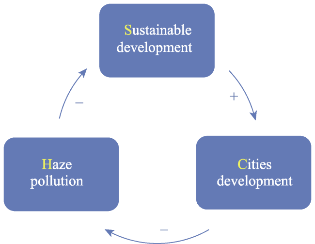
Fig. 1 The framework of city development and haze pollution

Note: “+” means positive impact, while the meaning of “-” is negative impact on haze pollution.

Ruan et al. (2020) suggested that a robust system should be established for city development where the government should develop implementable and flexible policies to achieve sustainable urban development. Yang et al. (2017) found that the sustainable development level is increasing in most cities in China. Zhang et al. (2019) investigated the “Five modernizations” in Chinese cities to provide insights into the sustainable development pathways and patterns for policymakers. Wang et al. (2021) examined the effects of moving window size and the scaling mechanism when analyzing urban expansion patterns. The results of that study show that a changing moving window size has varying impacts on delineating urban dynamics. To investigate the causes of haze pollution, domestic and foreign studies have conducted in-depth analyses of two aspects: natural factors and human activities (Kearsley and Riddel, 2010; Wooldridge, 2012; Vieira-Filho et al., 2015). China’s rapid urbanization has brought about spatial expansion, with the area of urban construction in China rising from 19504.6 km2 in 1997 to 56075.9 km2 in 2018. Therefore, USE is a very important issue in China. By considering the natural and socioeconomic variables, the Cellular automata model has been applied to examine the relationship between USE and its driving factors (Li et al., 2017). USE has led to significant changes in urban growth patterns in metropolitan areas (Dadashpoor et al., 2019), and the USE has transformed from a high-density sprawl on the urban fringe in the period of industrialization to modern diffusional expansion.
Studies investigating the impact of USE on atmospheric pollution are abundant (Pourahmad et al., 2007; Hien et al., 2020; Shi et al., 2020; Xu et al., 2021). The diffusion of urban air pollutants in “spread cities” is more serious than in compact cities in the United States (Stone, 2008). The more compact the city, the less the diffusion, and the easier it is to reduce the emission of pollutants. Therefore, a lack of good planning for the “spread cities” will lead to environmental degradation. USE has impacted transportation in 83 major cities in the United States (Ewing et al., 2003). The results of that study show that low-density and vehicle-oriented urban sprawl is not conducive to good air quality. The research on USE and haze pollution has only begun to emerge in recent years, and it has mainly focused on two aspects. On the one hand, some scholars believe that haze pollution is undoubtedly affected by the disorderly expansion of cities (Zhang et al., 2018). Urban sprawl increases greenhouse gas emissions and leads to increased emissions of suspended particulates (Glaeser and Kahn, 2004). Shi et al. (2019) suggested that in large cities, i.e., those with a population greater than 5 million and less than 10 million, the compactness of the city helps reduce the PM2.5 levels. Shi et al. (2021) found that urban spatial expansion could effectively explain the changes in the PM2.5 emissions from fossil fuel combustion in the central region. On the other hand, some scholars believe that USE will reduce haze pollution. For example, Cheng et al. (2017) reported that the denser the urban population in China, the more severe the haze pollution. Other studies, such as Juhee (2014), argued that the compact urban form was unsuitable for China because China already has high-density mixed urban land.
In summary, the existing literature on USE and haze pollution is insufficient, and there is still a lack of studies on the USE of China’s 29 provincial capitals. On the research scale, there is a lack of literature that examines the USE of China’s eight regions. From the perspective of research content, there is no consensus on the impact of USE on haze. In addition, there is also a lack of studies using the geographically weighted regression (GWR) model for analysis. GWR is a good way to explore this topic since it considers the spatial pattern elements, which can better reflect the impact of the spatial expansion of different cities and regions on haze pollution. Based on these shortcomings, this article intends to expand the footprint in three ways. Firstly, using the 29 provincial capital cities of China as samples to investigate the impact of USE on PM2.5, this study provides new evidence for the relationship between USE and haze in China. Secondly, the GWR model is used for empirical analysis because it is more significant for parameter estimation and statistical tests, and it has a smaller residual than the ordinary least squares (OLS) method. Thirdly, based on the vast territory of China, and differences in the endowments of resources and economic development conditions, the 29 Chinese cities are divided into eight regions for analysis. According to local conditions, strong operational policies and measures are proposed as a reference for the Chinese government. These findings will help us to understand the relationship between USE and haze, and provide valuable information for enabling planners and governments to formulate appropriate policies for scientifically-based city development. These are the main contributions of this research.

2 Background of urban spatial expansion

China’s urban space is expanding rapidly, with the area of urban construction in China rising from 19504.6 km2 in 1997 to 56075.9 km2 in 2018. China’s urban expansion is closely related to the local government’s land financing. The local governments of China not only have to bear the expenditures required for their operations, but they also need the corresponding income to promote local economic growth and provide public infrastructure for the citizens. Land financing has become a very important way for local governments to ease their financial pressure. Land financing mainly promotes land development in three ways which promote urban space expansion. First, the PCGDP-oriented local government assessment mechanism provides many incentives to attract investment. For example, the local government builds industrial parks and development zones by reducing the price of the land supply, attracting enterprises and capital to enter, promoting urban economic development, and obtaining promotion capital. Second, in order to make up for the cost of transferring industrial land at a low price, local governments will sell a large amount of commercial and residential land at high prices through listings, bidding, and auctions. Third, based on the convenience of transportation, local governments tend to build new residential areas and university towns in the suburbs, which has led to the continuous expansion of the urban space. In addition to land financing, urbanization is an important driver of urban expansion in China. China’s urbanization process is developing rapidly, and the level of urbanization exceeded 60% in 2019. A large proportion of the rural populations is concentrated in cities, and the demands for housing, schools, and commodities have increased. Cities have promoted the development of real estate investment, manufacturing, and service industries, so that the urban space continues to expand.
The expansion of urban space in China has exacerbated the problem of haze pollution. The expansion of urban space encroaches on nearby farmland, cultivated land, wetlands, and green spaces, weakening the inherent purification and regulatory capabilities of the ecological ring system. It prevents the ecosystem from absorbing and degrading air pollutants promptly, and urban space expansion increases the proportion of urban construction land area. Urban construction, such as building construction and real estate investment and development, will produce a lot of smoke and dust emissions, which will directly cause haze pollution problems. In addition, due to the expansion of the city, urban residents tend to live farther away from their place of work, so commuting distances increase, and commuting hours are extended. People will rely more on private cars for travel, and private cars will consume more petrochemical energy and produce exhaust emissions, especially PM2.5 emissions. In addition, urban expansion has shifted rural landless farmers from agricultural production departments to non-agricultural production departments. As the level of urban expansion increases, consumer demand for housing decorations, household appliances, and heating in winter increases, and the corresponding increases in household energy consumption, such as electricity and gas, causes haze pollution.

3 Model and methodology specification

3.1 Moran’s I

To illustrate the spatial agglomeration of PM2.5 in the 29 provincial capital cities in China, there are two common methods for spatial autocorrelation analysis: local and global spatial autocorrelation. The global Moran’s I (GMI) index, proposed by Moran (1950), is often used to solve global spatial autocorrelation. This index can reflect the spatial characteristics of the investigated objects such as spatial agglomeration, spatial dispersion, and spatial randomness. The GMI formula is expressed as:
$\begin{align} & \text{Moran}\text{s }I=\frac{n\sum\limits_{i=1}^{n}{\sum\limits_{j=1}^{n}{{{w}_{ij}}\left( {{x}_{i}}-\bar{x} \right)\left( {{x}_{j}}-\bar{x} \right)}}}{\sum\limits_{i=1}^{n}{\sum\limits_{j=1}^{n}{{{w}_{ij}}\sum\limits_{i=1}^{n}{{{\left( {{x}_{i}}-\bar{x} \right)}^{2}}}}}} \\ & \begin{matrix} \begin{matrix} {} & {} \\\end{matrix} & \begin{matrix} {} & {} \\\end{matrix} \\\end{matrix}=\frac{\sum\limits_{i=1}^{n}{\sum\limits_{j=1}^{n}{{{w}_{ij}}\left( {{x}_{i}}-\bar{x} \right)\left( {{x}_{j}}-\bar{x} \right)}}}{{{S}^{2}}\sum\limits_{i=1}^{n}{\sum\limits_{j=1}^{n}{{{w}_{ij}}}}} \\ \end{align}$
where the variance of the observations is denoted by ${{S}^{2}}=\frac{1}{n}\sum\limits_{i=1}^{n}{{{({{x}_{i}}-\bar{x})}^{2}}}$; $\bar{x}=\frac{1}{n}\sum\limits_{i=1}^{n}{{{x}_{i}}}$is the average of the observations of all space units; xi and xj represent the observations of the i-th and j-th space units, respectively; the total number of spatial units is denoted by n; and a spatial weight matrix is denoted as wij.
The value range of the GMI index is [-1, 1]. If GMI>0, a positive spatial autocorrelation is indicated, and the closer the index is to 1, the more clustered together the similar attributes are. If GMI<0, a negative spatial autocorrelation is indicated, and the closer the index is to -1, the more clustered together the different attributes are. If GMI=0, there is no spatial autocorrelation. In generating the GMI index, to further clarify the relevant numerical characteristics of the index, the expected value and variance are usually given.
The expected value of the GMI index is:
${{E}_{n}}GMI=-\frac{1}{n-1}$
The variance of the GMI index is:
$VA{{R}_{n}}GMI=\frac{{{n}^{2}}{{w}_{1}}+n{{w}_{2}}+3w_{0}^{2}}{{{w}^{2}}({{n}^{2}}-1)}-E_{n}^{2}GMI$
Where ${{w}_{0}}=\sum\limits_{i=1}^{n}{\sum\limits_{j=1}^{n}{{{w}_{ij}}}}$, ${{w}_{1}}=\frac{1}{2}\sum\limits_{i=1}^{n}{\sum\limits_{j=1}^{n}{({{w}_{ij}}}}+{{w}_{ji}}{{)}^{2}}$, ${{w}_{2}}=\sum\limits_{i=1}^{n}{{{({{w}_{i}}+{{w}_{j}})}^{2}}}$; and the sums of i rows and j columns in the spatial weight matrix are denoted as wi and wj, respectively. $E_{n}^{2}GMI$is the square of ${{E}_{n}}GMI$.
To verify the authenticity of the GMI index, a significance test is also performed. The z-score normal distribution hypothesis test is usually used. The z-test formula is:
$z=\frac{\text{Moran}\text{s }I-E(\text{Moran}\text{s }I)}{\sqrt{VAR(\text{Moran}\text{s }I)}}$
where E(Moran’s I) is the expected value of Moran’s I, VAR(Moran’s I) is the variance value of Moran’s I. Local spatial autocorrelation analysis can be illustrated by the Moran’s I index scatter plot. Anselin (1996, 2002) believed that the Moran’s I index scatter plot can visually show the situation of spatial autocorrelation. The Moran’s I index scatter plot is a two-dimensional visualization of (z, Wz), where z is a space lag factor, W is a spatial weight matrix, and Wz represents the weighted spatial calculation of the observations of the spatial unit. According to the four types of correlations, the Moran’s I index scatter plot is divided into four quadrants as H-H, L-H, L-L, and H-L, which illustrates the local spatial relationship between a corresponding spatial unit and its neighboring units. Among them, the first and third quadrants show the positive spatial correlation of observations, as the two regions have the same agglomeration characteristics. The first quadrant is in the form of a spatial connection in which the adjacent high-value spatial units surround a high-observation spatial unit. The third quadrant is for a low-observation spatial unit surrounded by adjacent low-value spatial units. On the other hand, the second and fourth quadrants explain the negative spatial correlations of observations, also known as spatial outliers, and indicate a sizeable spatial difference between the different observations and substantial spatial heterogeneity. The second quadrant is for a low-observation spatial unit surrounded by adjacent high-value spatial units; while the fourth quadrant is for a high-observation spatial unit surrounded by adjacent low-value spatial units.

3.2 Geographically weighted regression model

The classical linear regression method assumes that the variables’ observations are randomly sampled in space, and the relationship between the variables does not change with changes in geographic location. However, this assumption leads to some bias, which masks the local characteristics of the relationship between variables, and the global result is the average effect of the different regions (Zhou et al., 2019). Therefore, the GWR method is needed to analyze the factors influencing haze pollution in different regions. In addition, the GWR can solve the problem of the spatial autocorrelation error term in the OLS model (Quan, 2005).
The classical (global) linear regression model (Xu and Lin, 2017) is:
${{y}_{i}}={{\beta }_{0}}\text{+}\sum\limits_{j=1}^{n}{{{x}_{ij}}}{{\beta }_{j}}+{{\xi }_{i}},\text{ }i=1,2,\cdots,m,\text{ }j=1,2,\cdots,n$
where the coefficient ${{\beta }_{0}}$ is a constant, parameter β is estimated in the OLS model, and a random error term is denoted by ξ.
The GWR model that extends the general linear regression model is:
${{y}_{i}}={{\beta }_{0}}\text{(}{{u}_{i}}\text{,}{{v}_{i}}\text{)+}\sum\limits_{j=1}^{k}{{{\beta }_{j}}}({{u}_{i}}\text{,}{{v}_{i}}\text{)}{{x}_{ij}}+{{\xi }_{i}}$
In this equation, the coefficient ${{\beta }_{j}}$ changes with a change in the local geographic location i in space, and a local regression estimation is used instead of the constant β0 (which is used in the global estimation method). The number of parameters to be estimated is denoted by j; the latitude and longitude of the i-th point in space is denoted by (ui, vi); βj(ui, vi) represents the j-th regression parameter of the i-th sample point in space and it is a function of geographic location (i.e., latitude and longitude); and the random error term for the i-th area is denoted by ξi.
The log-likelihood function of equation (6) is:
$\begin{align} & \lg L=L[{{\beta }_{0}}\text{(}u\text{,}v\text{),}\cdots \text{,}{{\beta }_{k}}\text{(}u,v)|M] \\ & =-\frac{1}{2{{\sigma }^{2}}}\sum\limits_{i=1}^{n}{[{{y}_{i}}}-{{\beta }_{0}}({{u}_{i}},{{v}_{i}})-\sum\limits_{j=1}^{k}{{{\beta }_{k}}}({{u}_{i}}\text{,}{{v}_{i}}\text{)}{{x}_{i}}{{]}^{2}}+\alpha \\ \end{align}$
where lg is logarithmic likelihood function; $\alpha $ is a constant term; and $M=[{{y}_{i}},\text{ }{{x}_{ij}},({{u}_{i}},{{v}_{i}}),\ i=1,2,\cdots,n,\ \text{ }j=1,2,\cdots,k]$, the latitude and longitude of a geographic location are denoted by u and v, respectively. Hastie and Tibshirani (1993) proposed a local method to estimate the parameter β as:
$\hat{\beta }\text{(}{{u}_{i}}\text{,}{{v}_{i}}\text{)=(}{X}'W({{u}_{i}}\text{,}{{v}_{i}}\text{)}X{{)}^{-1}}\text{(}{X}'W({{u}_{i}}\text{,}{{v}_{i}}\text{)}Y)$
Where $\hat{\beta }$ is the estimator of β; X is the explanatory variable vector; X' is derivation of X; and Y is the explained variable; W(ui,vi) is an n×n diagonal matrix with diagonal elements Wij. As the spatial weight matrix W(ui,vi) changes, $\hat{\beta }$ is a weighted least squares estimation. Wij is usually determined by latitude and longitude. The spatial weight matrix W(ui,vi) mainly includes the following three calculation methods
Gaussian distance: ${{W}_{ij}}=\phi ({{d}_{ij}}/\sigma \theta )$
where the bandwidth is denoted by θ; dij is the distance between the space unit i and j; $\theta$ represents the standard density; and the standard deviation of the distance vector is denoted by σ.
Exponential distance: ${{W}_{ij}}=\sqrt{\exp (-{{d}_{ij}}/\theta )}$
Cubic distance:${{W}_{ij}}={{[1-{{({{d}_{ij}}/{{q}_{ij}})}^{3}}]}^{3}}I({{d}_{i}}-{{q}_{i}})$
where the distance between the i-th region and the q-th neighboring region is denoted by qi, and a conditional function is denoted by I(di-qi). When the bandwidth is determined, a regression coefficient can be obtained. The cross-validation (cv) method is generally used to determine the bandwidth:
$cv=\sum\limits_{i=1}^{n}{{{\left[ {{y}_{i}}-{{{\hat{y}}}_{\ne i}}(\theta ) \right]}^{2}}}$
where the fitted value of yi is denoted by ${{\hat{y}}_{\ne i}}$; and the bandwidth is denoted by θ when cv is minimum.

3.3 Model specification

To illustrate the impact of USE on haze, the following regression model is set:
$\begin{align} & \ln P{{M}_{2.5i}}={{\beta }_{1}}\ln CL{{A}_{i}}+{{\beta }_{2}}\ln PCGD{{P}_{i}}+{{\beta }_{3}}\ln GS{{P}_{i}}+ \\ & \ \ \ \ \ \ \ \ \ \ \ \ \ \ \ \ {{\beta }_{4}}\ln DP{{I}_{i}}+{{\beta }_{5}}\ln CO{{N}_{i}}+{{\xi }_{i}} \\ \end{align}$
where i represents a provincial capital city; PM2.5i is the PM2.5 concentration of city i, which refers to haze pollution (μg m‒3); CLA stands for USE; PCGDP refers to per capita income; GSP refers to urban greening level; DPI refers to per capita disposable income of the urban residents; CON refers to the per capita consumption expenditure of the urban residents; β15 are the elastic coefficients to be estimated; and ξi is a random error term.
Adding a spatial position element variable to equation (13), the specific model of GWR becomes:
$\begin{align} & \ln \text{P}{{\text{M}}_{2.5i}}=\ln {{\beta }_{0}}({{u}_{i}},{{v}_{i}})+{{\beta }_{1}}({{u}_{i}},{{v}_{i}})\ln CL{{A}_{i}}+ \\ & \ \ \ \ \ \ \ \ \ \ \ \ \ \ \ \ {{\beta }_{2}}({{u}_{i}},{{v}_{i}})\ln PCGD{{P}_{i}}+{{\beta }_{3}}({{u}_{i}},{{v}_{i}})\ln GS{{P}_{i}}+ \\ & \ \ \ \ \ \ \ \ \ \ \ \ \ \ \ \ {{\beta }_{4}}({{u}_{i}},{{v}_{i}})\ln DP{{I}_{i}}+{{\beta }_{5}}({{u}_{i}},{{v}_{i}})\ln CO{{N}_{i}}+{{\xi }_{i}} \\ \end{align}$
where the latitude and longitude of the i-th point in space are denoted as ui and vi, respectively, and the parameter β is a function of ui and vi.

3.4 Data sources and variables

This study examines 29 provincial capitals in China (excluding Taiwan, Macao, and Hong Kong). Lhasa and Urumqi are not included because of the lack of data. According to the location characteristics of the provincial capitals, the studied cities are divided into eight regions as shown in Table 1. The PM2.5 data are from the China Statistical Yearbook 2018. The urban construction area and green space per capita are from the China Urban Construction Statistical Yearbook 2017. The GDP per capita data are from the China City Statistical Yearbook 2018. Disposable income per capita (DPI) and consumption expenditure per capita (CON) are from the Statistical Communiqué 2017 on the National Economic and Social Development of Cities. The definitions and descriptive statistics of the variables in this study are shown in Tables 2 and 3.
Table 1 Distribution of the 29 provincial captical cities in the eight areas of China
Region Cities Region Cities
Eastern coast Hangzhou (HZ), Shanghai (SH), Nanjing (NJ) Middle Reaches of the Yangtze
River
Nanchang (NC), Hefei (HF), Changsha (CS), Wuhan (WH)
Northern coast Beijing (BJ), Shijiazhuang (SJZ), Jinan (JN), Tianjin (TJ) Middle Reaches of the Yellow River Taiyuan (TY), Hohhot (HHHT), Xi’an (XA), Zhengzhou (ZZ)
Southern coast Fuzhou (FZ), Haikou (HK), Guangzhou (GZ) Southwest region Nanning (NN), Guiyang (GY), Kunming (KM), Chongqing (CQ), Chengdu (CD)
Northeast region Harbin (HRB), Changchun (CC), Shenyang (SY) Northwest region Yinchuan (YC), Xining (XN), Lanzhou (LZ)
Table 2 Definitions of the explanatory and dependent variables
Variable Definition Units
PM2.5 Fine particulate matter, Annual average concentration μg m-3
CLA Area of urban construction land km2
PCGDP Per capita GDP yuan
GSP Public recreational green space per capita m2
DPI Per capita disposable income of urban residents yuan
CON Per capita consumption expenditure of urban residents yuan
Table 3 Statistics of the variables
Variable PM2.5 CLA PCGDP GSP DPI CON
Mean 48.482 564.765 101205.3 13.538 40781.40 27458.02
Median 48.000 446.000 94477.0 12.920 38536.00 25852.00
Maximum 86.000 1910.740 152441.0 22.670 62596.00 42304.00
Minimum 20.000 89.670 61589.00 7.580 30043.00 17279.00
Std. Dev. 14.857 410.486 26917.71 3.347 9383.099 6507.272
Sum 1406.000 16378.20 2934955 392.610 1182661 796282.7

4 Empirical research

4.1 Multicollinearity test

The spatial correlation and multicollinearity test results of the variables are listed in Table 4. While the correlation coefficients between disposable income per capita of urban residents, GDP per capita, and consumption expenditure per capita are greater than 0.8, the correlation coefficients between other variables are lower than 0.68 (so some have not passed the significance test). Further testing for multicollinearity using a variation expansion factor (VIF) indicated that the VIF values were greater than 1 and less than 8, with an average value of 3.36. Since the VIF values are lower than 10, indicating that no multicollinearity exists among the independent variables, the next analysis can be performed.
Table 4 The correlation coefficient matrix
Variables VIF lnPM2.5 lnCLA lnPCGDP lnGSP lnDPI lnCON
lnPM2.5 1
lnCLA 1.433 0.346* 1
lnPCGDP 2.984 0.104 0.468** 1
lnGSP 1.071 ‒0.085 ‒0.058 ‒0.089 1
lnDPI 7.153 0.024 0.596*** 0.801*** 0.048 1
lnCON 4.182 ‒0.042 0.542*** 0.676*** ‒0.006 0.884*** 1

Notes: * means P < 0.10, ** means P < 0.05, *** means P < 0.01.

4.2 Spatial distributions of urban haze pollution and spatial expansion

Using ArcGIS 10.2 software and the Jenks natural breakpoint method, the PM2.5 concentration distribution map of the 29 provincial capitals in 2017 was drawn. The average concentrations of PM2.5 are divided into five levels from low to high. The cities in the first tier are Haikou, Fuzhou, and Kunming. The second-tier cities are Guiyang, Xining, Guangzhou, Nanning, Shanghai, Nanjing, and Nanchang. The cities located in the third tier include Hohhot, Hangzhou, Chongqing, Changchun, Yinchuan, Lanzhou, Shenyang, Wuhan, and Changsha. The fourth-tier cities are Chengdu, Hefei, Beijing, Harbin, Tianjin, Taiyuan, Jinan, and Zhengzhou. The fifth-tier cities are Xi’an and Shijiazhuang.
The degrees of USE are divided into five levels from low to high. The cities in the first tier are Xining, Haikou, and Yinchuan. The second-tier cities are Hohhot, Shijiazhuang, Fuzhou, Nanning, Nanchang, Lanzhou, Changsha, Taiyuan, and Guiyang. The cities located in the third tier include Harbin, Kunming, Hefei, Jinan, Zhengzhou, Changchun, Hangzhou, Shenyang, Xi’an, and Guangzhou. The fourth-tier cities are Chongqing, Nanjing, Chengdu, Wuhan, and Tianjin. The fifth-tier cities are Beijing and Shanghai.
In summary, PM2.5 and spatial expansion showed spatial heterogeneity in 2017 among the 29 provincial capitals in China. Furthermore, PM2.5 has a certain correlation with urban spatial expansion. Cities with low spatial expansion, such as Haikou, also have low haze pollution. Some cities with a high degree of spatial expansion, such as Tianjin, Beijing and Chengdu, also have a high degree of haze pollution.

4.3 Global and local spatial correlation analysis

Using the threshold distance weight and Monte Carlo test (999 permutations) method, we calculated the GMI index values of PM2.5 in the 29 provincial capitals in China in 2017 (Fig. 2). The Moran’s I index passed the significance test at the 5% level, indicating that there is significant spatial autocorrelation of PM2.5 in those capital cities. First, 17 provincial capitals are located in the first and third quadrants, which mean H-H or L-L agglomeration. Among them, seven cities mainly located on the Northern coast (NC) and the MYR, namely Beijing, Shijiazhuang, Taiyuan, Jinan, Zhengzhou, Tianjin, and Wuhan, are located in the first quadrant, so they are high-high clusters. Ten cities mainly located in the Southern coast and EC, including Hangzhou, Nanchang, Shanghai, Nanjing, Fuzhou, Haikou, Guiyang, Kunming, Guangzhou, and Nanning, are located in the third quadrant, which indicates an L-L cluster. Furthermore, another 12 cities are located in the second and fourth quadrants. Among them, the five cities of Changchun, Hohhot, Yinchuan, Xining, and Chongqing are located in the second quadrant; while the seven cities of Shenyang, Xi’an, Chengdu, Changsha, Harbin, Hefei, and Lanzhou are in the fourth quadrant. These patterns show that the geographic distribution of PM2.5 in different provincial capitals in China exhibits a trend of agglomeration.
Fig. 2 Moran scatter plot of PM2.5 in the 29 provincial capital cities in China

Note: Negative values in the coordinate axis indicate the direction of change.

4.4 GWR regression results

As described in Section 3.3, strong spatial autocorrelations of haze exist in Chinese capitals, and the spatial differences are obvious. To study the impacts of factors such as USE on the haze pollution in different cities, this study uses the GWR model for analysis. The GWR model parameter includes three methods: Exponential, Gaussian, and Tricube weight decay function. In the estimation of the GWR model, the choice of bandwidth is particularly important because a large bandwidth will lead to a large deviation of the regression parameters, while a small bandwidth will result in a large variance of the parameters. In choosing the bandwidth, there are generally minimum cv and minimum AIC methods. This study uses the minimum cv method to determine the optimal bandwidth. Matlab R2014a was used to obtain the results shown in Table 5.
Table 5 The overall fitting results of the GWR model
Weight decay type Exponential Gaussian Tricube
Explained variable lnPM2.5 lnPM2.5 lnPM2.5
R2 0.9899 0.9540 0.6090
Adjusted R2 0.9878 0.9444 0.5276
Bandwidth 4.4721 0.8169
Observation 29 29 29
As shown in Table 5, the estimated R2 values of the three-parameter methods of Exponential, Gaussian, and Tricube function are 0.9899, 0.9540, and 0.6090, respectively; and the adjusted R2 values are 0.9878, 0.9444, and 0.5276, respectively. Since the exponential GWR model estimated R2 and adjusted R2 values are among the highest, this study chose that model for analysis. The optimal bandwidth determined by the minimum cv is 4.4721. The GWR model estimation results based on the exponential method are shown in Table 6. It can be seen that USE, PCGDP, greening level, disposable income, and consumption expenditure are significant at the level of 10% or above. However, different regions and explanatory variables have different effects on haze pollution.
Table 6 Estimation results of the GWR model based on exponential functions
Region City Constant lnCLA lnPCGDP lnGSP lnDPI lnCON
SC
(Southern coast)
FZ 7.386* 0.433*** 1.042*** ‒0.272* ‒2.938*** 1.329***
HK ‒7.449*** 0.466*** ‒0.891*** ‒0.960*** 2.533*** ‒0.575***
GZ 7.559** 0.416*** 0.738** ‒0.413*** ‒1.620*** 0.325
NC
(Northern coast)
BJ 14.160*** 0.204** ‒0.652** 0.035 0.108 ‒0.491
SJZ 17.562*** 0.248*** ‒1.215*** ‒0.174 ‒0.079 0.031
JN 12.767*** ‒0.022 ‒0.632*** 0.165 ‒0.698* 0.568
TJ 11.632*** 0.096 ‒0.395 0.166 ‒0.014 ‒0.372
EC
(Eastern coast)
HZ 8.092** 0.391*** 0.990*** 0.371 ‒3.812*** 2.104***
SH 12.681*** ‒0.080 ‒0.287 0.123 ‒1.354** 0.909*
NJ 12.101*** 0.162 0.105 0.208 ‒2.392*** 1.426**
NE
(Northeast)
HRB 40.476*** 0.959*** ‒0.137 0.409*** 5.649*** ‒9.924***
CC 21.059* 0.330 0.127 0.271* 4.072*** ‒6.276***
SY 7.670 ‒0.035 0.309 0.293** 1.985*** ‒2.800**
MYTR
(Middle Reaches of the Yangtze River)
NC 10.307*** 0.395*** 0.709** ‒0.138 ‒2.764*** 1.234***
HF 12.231*** 0.237** 0.158 0.120 ‒2.452*** 1.390**
CS 10.360*** 0.294*** 0.705** ‒0.280** ‒2.087*** 0.620*
WH 12.082*** 0.258** 0.167 ‒0.132 ‒2.040*** 1.013**
MYR
(Middle Reaches of the Yellow River)
TY 17.356*** 0.300*** ‒1.271*** ‒0.183 0.240 ‒0.250
HHHT 18.442*** 0.404*** ‒1.334*** 0.001 0.386 ‒0.549*
XA 5.551 0.001 ‒0.888** ‒0.615** 2.270*** ‒1.349**
ZZ 14.079*** 0.062 ‒0.793*** ‒0.124 ‒0.341 0.269
NW
(Northwest)
YC 9.938*** 0.309*** ‒0.970* 0.098 1.795** ‒1.565***
XN ‒18.923*** 0.008 ‒0.921* ‒0.120 1.873** 1.387**
LZ ‒12.603** 0.067 ‒0.781 ‒0.196 1.859** 0.603
SW
(Southwest region)
NN ‒7.845*** 0.473*** ‒0.942*** ‒0.975*** 2.635*** ‒0.583***
GY ‒8.724*** 0.486*** ‒0.845*** ‒0.959*** 2.641*** ‒0.622***
KM ‒14.612*** 0.562*** ‒0.862* ‒1.186*** 3.310*** ‒0.701***
CQ ‒1.480 0.324*** ‒0.293 ‒0.796** 1.780** ‒0.993*
CD 5.556*** 0.207*** ‒0.428 ‒1.039** 2.496*** ‒2.136**

Notes: * means P < 0.10, ** means P < 0.05, *** means P < 0.01.

5 Discussion

As different explanatory variables such as regions and USE have different impacts on haze pollution, it is necessary to provide in-depth discussions of these differences.

5.1 Impact of urban spatial expansion on haze pollution

The spatial expansion of most cities has a significant positive effect on haze pollution, i.e., the USE will increase the degree of haze pollution, but it has different impacts on different regions. From the perspective of the cities, the spatial expansion of Harbin has the most significant impact on haze pollution, with a value of 0.959, i.e., for each percentage of spatial expansion in Harbin, the haze will increase by 0.959 percent. Beijing’s spatial expansion has the smallest impact on haze pollution at 0.204. The elasticity coefficient of Harbin’s spatial expansion is 4.7 times that of Beijing. This is because Beijing, as the capital, has a greater degree of government intervention. The measures taken in the process of spatial expansion are stricter and more orderly, so the impact on haze pollution is smaller.
Among the different regions, the spatial expansion of each city in the three regions of the SW, the SC, and the MYTR passed the significance test, i.e., the spatial expansion of each city in these three regions will have a significant positive effect on haze. Therefore, we must focus on controlling urban expansion in these three regions to avoid the adverse impacts of haze pollution. Among them, the coefficient of spatial expansion of the SC cities is the largest at 0.438, followed by the SW at 0.4104, and finally, the MYTR at 0.296. In addition, the urban expansion of two cities on the NC and the MYR passed the significance test while only one city on the EC, the NW, and the NE passed the significance test, indicating that the impacts of spatial expansion on the haze pollution are minimal in these three regions.

5.2 Impact of economic development on haze pollution

The impact of economic development on haze pollution is more interesting, as it can be positive or negative, or it may fail the significance test in different cities. The economic development of Fuzhou, Guangzhou, Hangzhou, Nanchang, and Changsha has a significant positive impact on haze pollution; however the economic development of Haikou, Beijing, Shijiazhuang, Jinan, Taiyuan, Hohhot, Xi’an, Zhengzhou, Yinchuan, Xining, Nanning, Guiyang, and Kunming has a significant negative impact, i.e., the economic development of these cities will reduce the degree of haze pollution. Regionally, the impact of the economic development of the SC cities on haze passed the significance test, but in two cities it has a positive impact on haze pollution while it has a negative impact in one other city. The economic development of each city in the MYR has a significant negative impact on haze pollution, indicating that the economic development in the region will reduce the degree of haze pollution. There are three cities in the NC, two cities in the NW, and three cities in the SW for which the impact of urban economic development on haze pollution is significantly negative. Cities with high levels of economic development tend to have a strong sense of governmental pollution control and will invest more in environmental protection. Moreover, they also have more clean energy vehicles than high-emission vehicles. Finally, the economic development of one city on the EC and two cities in the MYTR has a significant positive impact on haze pollution.

5.3 Impact of urban greening level on haze pollution

Of the 29 cities, the impact of the greening level on haze passed the significance test in 13 cities, with obvious regional characteristics. Fuzhou and Haikou have significantly negative greening coefficients. The impact of greening levels on haze in some cities is not significant, which indicates that these cities have not played their due role in reducing haze. From the regional perspective, the greening level of each city in the SC and the SW has a significant negative impact on haze, i.e., an increase in greening level will reduce the level of haze. The impact of the urban greening level on the haze in Xi’an in the MYR and the cities in the MYTR is also significantly negative. This pattern shows that “urban greening” can effectively adsorb, block, and degrade atmospheric particulates and it plays a role in purifying the air and resisting haze (Hastie and Tibshirani, 1993). However, the impact of urban greening on haze in the NE is significantly positive. This is because of the extremely cold climate in the NE. On the one hand, trees shed all their leaves in autumn and winter, so they cannot effectively adsorb PM2.5 particles floating in the atmosphere. On the other hand, the extended use of heating aggravates the haze due to the cold climate from October to May of the following year in the NE, i.e., the use of heating equipment lasts for eight months a year. Thus, the higher energy consumption contributes to haze pollution.

5.4 Impact of urban resident disposable income on haze pollution

The impact of urban resident disposable income on haze in most cities passed the significance test. The rising disposable income of residents in all cities along the EC and the MYTR has a negative impact on haze pollution and passed the significance test. The SC cities of Fuzhou and Guangzhou, and the NC city of Jinan are the same as the above two regions, which is consistent with the conclusions of Liang et al. (2019). This is because the high-income residents have loose budgets and are more willing to purchase green electricity than low-income residents (Xie and Zhao, 2018). However, the increase in disposable income of urban residents in the NE, NW, and SW will increase the haze pollution because the disposable income of residents in these three regions is low, ranking sixth, eighth, and seventh among the eight regions. That is, the disposable income of residents in these areas is low and environmental protection awareness is weak, so the investment in haze management is also low.

5.5 Impact of urban resident consumption expenditure on haze pollution

The consumption expenditure of residents in the NE, SW, and in Hohhot and Xi’an in the MYR has a negative impact on haze. That is, the increase in residential consumer spending in these areas will cause a reduction in the haze. This is because consumer spending in these areas is relatively low. For example, the consumer spending levels in the MYR and the SW rank seventh and sixth. These rankings put residents in these areas at a relatively low level of consumption of cars and other vehicles, which has a negative impact on haze pollution. For these regions, measures should be taken to increase consumption. In contrast, the rising consumption of urban residents in the MYTR and the EC will cause the haze levels in those regions to increase. The consumption expenditure of residents in these two areas has reached a high level. For example, the consumption expenditure of residents on the EC ranks first among the eight regions, so the consumption demand of residents for automobiles and gasoline is higher, resulting in higher haze pollution.
Household consumption, especially urban household consumption, is another crucial source of haze (Yang et al., 2019). In a long-term study, You et al. (2017) found that the decrease of PM2.5 by 20% in Shanghai in one month was significantly related to a 2.2% reductionin residential electricity consumption.

6 Conclusions

This study used the GWR method to analyze the impact of USE on haze. This analysis found that the spatial expansion of most cities has a significant positive impact on haze pollution, i.e., USE aggravates the degree of haze, but the impacts differ regionally. The expansion of urban space along the SC, the MYTR, and the SW will have a significant positive impact on haze. Among them, the coefficient of spatial expansion of the SC cities is the largest at 0.438, followed by the SW at 0.4104, and finally the MYTR at 0.296. To take into account the city’s efforts toward development and the control of haze pollution, we propose some policies for the reference of the Chinese government.

7 Policies

7.1 Strengthening regional cooperation

There are significantly positive spatial autocorrelations in haze pollution between the Chinese capital cities. For example, low-low agglomeration is mainly located in the SC and EC; while high-high agglomeration is mainly located in the NC and the MYR. Therefore, to control haze pollution, the government should further strengthen environmental regulations, focusing on strengthening the environmental regulations on the NC and the MYR, through the introduction of relevant policies and measures to prevent further increases in haze pollution. At the same time, it should strengthen regional cooperation, e.g., cities in the NC and the MYR should exchange information on haze pollution, share resources, coordinate pollution management, and eventually achieve mutual benefits.

7.2 Reasonably control the spatial expansion of cities, especially in the SC, the MYTR, and the SW

From the perspective of the cities, the impact of USE on haze is significantly positive in most cities, indicating that USE will bring haze pollution problems. This is because an increase in building construction sites accompanies the expansion of urban space, and the large amount of dust formed by housing and municipal construction is one of the main sources of haze pollution in Chinese cities (Banzhaf and Lavery, 2010). At the same time, the expansion of urban space will increase the length of roads, the distance between work and residence, the use of vehicles and other means of transportation, and the consumption of petroleum, and automobile exhaust emissions are the primary source of haze pollution. In this case, high-density and compact urban forms can help to reduce haze pollution. Therefore, we must scientifically formulate urban development plans, effectively manage urban space, build compact cities, and avoid disorderly urban sprawl. Also, the development of electric vehicles, green buildings, solar photovoltaic wind energy, and biotechnology industries can contribute to haze reduction (Chang and Lee, 2016). Meanwhile, residents should also be encouraged to use low-energy vehicles and electric vehicles to reduce exhaust emissions. In addition, different policies should be adopted depending on the size of the city, such as a single-center urban structure for small and medium-sized cities. To reduce traffic distances and traffic congestion, large cities should develop a polycentric urban structure. The spatial expansion of each city in the SC, the MYTR, and the SW has a significant positive impact on haze. Therefore, we must focus on controlling the expansion of urban space in these three regions, laying out the urban infrastructure in these three areas rationally, implementing refined management, and reducing their haze concentrations.

7.3 The acceleration of economic development is needed in the SW, MYR, NC, and NW

The economic development of the MYR, NC, NW, and SW regions will reduce haze pollution. Therefore, these four regions must accelerate their economic development since their current levels are relatively low among the capital cities in the country. For example, the GDP per capita of the MYR and the NC rank fourth and fifth, respectively, and those of the NW and SW rank eighth and sixth, respectively. In the context of China’s overall progress in building a strong country through science and technology, these regions can accelerate their economic development by improving their technological innovation capabilities. Science and technology are the primary productive forces. Advances in science and technology can not only increase productivity and total economic development but also change the mode of economic development and allow them to achieve intensive growth. Therefore, these four regions should improve their technological innovation capabilities through talent introduction and other methods, thereby increasing the speed of economic development.

7.4 Strengthening urban greening

It is necessary to strengthen urban greening in order to reduce haze pollution. Firstly, by increasing the investment in greening and expanding urban greening areas, the expansion of the green space will cover the bare land and effectively adsorb PM2.5 particles in the atmosphere. At the same time, plants can absorb pollutant gases and purify the environment by means of “natural regeneration”. Therefore, it is necessary to expand the scope of urban greening. By expanding the area of green space, improving the spatial balance of the greenspace will help to reduce the PM2.5 concentration and heat island effects because the urban green space can purify air and adsorb particulates (Groenewegen et al., 2012). Green belts and green buildings can help reduce pollution emissions, and Singapore is the best example of cultivating plants on the rooftops, which will beautify the city and adsorb pollutants. For the NE, garden plants should be planted to reduce haze pollution, forming a multi-level plant configuration structure so that the greening can play a role in purifying the air and reducing the concentration of atmospheric particulates.

7.5 Increasing consumer spending in the NE, SW, and MYR, and environmental awareness and green consumption in the EC and the MYTR

The consumption expenditure of urban residents in the NE, the SW, and the MYR has a negative impact on haze pollution. For these regions, measures should be taken to increase consumption. On August 27, 2019, China issued “The Opinions on Accelerating the Development of Circulation and Promoting Commercial Consumption” which proposed 20 policies and measures to stabilize consumer expectations and boost consumer confidence. Accelerating the implementation of these 20 consumption measures will help to increase consumer spending in the three lowest regions. However, the rising consumption of urban residents in the EC areas and the MYTR will cause their haze pollution levels to rise. Thus, these two regions should adopt green consumption (Arli et al., 2018) and the government can adequately guide and encourage residents to use energy-efficient equipment. To ensure the continuity of related measures, energy, coal, fuel, and transportation taxes can be levied on the residents. Finally, efforts should be made to strengthen the education on energy-saving consumption for the younger generation, incorporate energy-saving and environmental protection materials into textbooks, and enable urban residents to establish energy-saving concepts from an early age.
[1]
Anselin L. 1996. The Moran scatterplot as an ESDA tool to assess local instability in spatial association. London, UK: Taylor & Francis.

[2]
Anselin L. 2002. Under the hood issues in the specification and interpretation of spatial regression models. Agricultural Economics, 27(3): 247-267.

DOI

[3]
Arli D, Tan L P, Tjiptono F, et al. 2018. Exploring consumers’ purchase intention towards green products in an emerging market: The role of consumers’ perceived readiness. International Journal of Consumer Studies, 42(4): 389-401.

DOI

[4]
Banzhaf H S, Lavery N. 2010. Can the land tax help curb urban sprawl? Evidence from growth patterns in Pennsylvania. Journal of Urban Economics, 67(2): 169-179.

DOI

[5]
Chang C T, Lee H C. 2016. Taiwan’s renewable energy strategy and energy-intensive industrial policy. Renewable and Sustainable Energy Reviews, 64: 456-465.

DOI

[6]
Chen Z, Wang J N, Ma G X, et al. 2013. China tackles the health effects of air pollution. Lancet, 382(9909): 1959-1960.

DOI PMID

[7]
Cheng Z H, Li L S, Liu J. 2017. Identifying the spatial effects and driving factors of urban PM2.5 pollution in China. Ecological Indicators, 82: 61-75.

DOI

[8]
Dadashpoor H, Azizi P, Moghadasi M. 2019. Analyzing spatial patterns, driving forces and predicting future growth scenarios for supporting sustainable urban growth: Evidence from Tabriz metropolitan area, Iran. Sustainable Cities and Society, 47: 101502. DOI: 10.1016/j.scs.2019.101502.

[9]
Ewing R, Pendall R, Chen D. 2003. Measuring sprawl and its transportation impacts. Transportation Research Record: Journal of the Transportation Research Board, 1831(1): 175-183.

DOI

[10]
Gao M, Guttikunda S K, Carmichael G R, et al. 2015. Health impacts and economic losses assessment of the 2013 severe haze event in Beijing area. Science of the Total Environment, 511: 553-561.

DOI

[11]
Glaeser E L, Kahn M E. 2004. Sprawl and urban growth (Chapter 56). Dublin, Ireland: Taylor & Francis.

[12]
Groenewegen P P, van den Berg A E, Maas J, et al. 2012. Is a green residential environment better for health? if so, why? Annals of the Association of American Geographers, 102(5): 996-1003.

DOI

[13]
Hastie T, Tibshirani R. 1993. Varying-coefficient models. Journal of the Royal Statistical Society: Series B (Methodological), 55(4): 757-779.

[14]
Hien P D, Men N T, Tan P M, et al. 2020. Impact of urban expansion on the air pollution landscape: A case study of Hanoi, Vietnam. Science of the Total Environment, 702: 134635. DOI:10.1016/j.scitotenv.2019.134635.

[15]
Juhee P. 2014. Effects of compact city form on transportation energy consumption and air pollution—Focusing on the major cities in Korea. Diss., Beijing, China: Tsinghua University. (in Chinese)

[16]
Kearsley A, Riddel M. 2010. A further inquiry into the pollution haven hypothesis and the environmental Kuznets curve. Ecological Economics, 69(4): 905-919.

DOI

[17]
Li C, Zhao J, Xu Y. 2017. Examining spatiotemporally varying effects of urban expansion and the underlying driving factors. Sustainable Cities and Society, 28: 307-320.

DOI

[18]
Liang L W, Wang Z B, Li J X. 2019. The effect of urbanization on environmental pollution in rapidly developing urban agglomerations. Journal of Cleaner Production, 237: 117649. DOI: 10.1016/j.jclepro.2019.117649.

[19]
MacKerron G, Mourato S. 2009. Life satisfaction and air quality in London. Ecological Economics, 68(5): 1441-1453.

DOI

[20]
Moran P A P. 1950. Notes on continuous stochastic phenomena. Biometrika, 37: 17-23.

PMID

[21]
Pourahmad A, Baghvand A, Zanganeh S, et al. 2007. The impact of urban sprawl up on air pollution. International Journal of Environmental Research, 1(3): 252-257.

[22]
Ruan F L, Yan L, Wang D. 2020. The complexity for the resource-based cities in China on creating sustainable development. Cities, 97: 102571. DOI: 10.1016/j.cities.2019.102571.

[23]
Shi K F, Shen J W, Wang L, et al. 2020. A multiscale analysis of the effect of urban expansion on PM2.5 concentrations in China: Evidence from multisource remote sensing and statistical data. Building and Environment, 174: 106778. DOI: 10.1016/j.buildenv.2020.106778.

[24]
Shi K F, Wang H, Yang Q Y, et al. 2019. Exploring the relationships between urban forms and fine particulate (PM2.5) concentration in China: A multi-perspective study. Journal of Cleaner Production, 231: 990-1004.

DOI

[25]
Shi K F, Wu Y Z, Li L Y. 2021. Quantifying and evaluating the effect of urban expansion on the fine particulate matter (PM2.5) emissions from fossil fuel combustion in China. Ecological Indicators, 125: 107541. DOI: 10.1016/j.ecolind.2021.107541.

[26]
Stone B J. 2008. Urban sprawl and air quality in large US cities. Journal of Environmental Management, 86(4): 688-698.

PMID

[27]
Vieira-Filho M S, Lehmann C, Fornaro A. 2015. Influence of local sources and topography on air quality and rainwater composition in Cubatão and São Paulo, Brazil. Atmospheric Environment, 101: 200-208.

DOI

[28]
Wang R, Feng Y J, Tong X H, et al. 2021. Impacts of spatial scale on the delineation of spatiotemporal urban expansion. Ecological Indicators, 129: 107896. DOI: 10.1016/j.ecolind.2021.107896.

[29]
Wooldridge J. 2012. Introductory econometrics:A modern approach. Boston, USA: South-Western Cengage Learning.

[30]
Xie B C, Zhao W. 2018. Willingness to pay for green electricity in Tianjin, China: Based on the contingent valuation method. Energy Policy, 114: 98-107.

DOI

[31]
Xu B, Lin B Q. 2017. Factors affecting CO2 emissions in China’s agriculture sector: Evidence from geographically weighted regression model. Energy Policy, 104: 404-414.

DOI

[32]
Xu X B, Xu Y, Xu H C, et al. 2021. Does the expansion of highways contribute to urban haze pollution? —Evidence from Chinese cities. Journal of Cleaner Production, 314: 128018. DOI: 10.1016/j.jclepro.2021.128018.

[33]
Yang B, Xu T, Shi L Y. 2017. Analysis on sustainable urban development levels and trends in China’s Cities. Journal of Cleaner Production, 141: 868-880.

DOI

[34]
Yang J, Song D, Fang D L, et al. 2019. Drivers of consumption-based PM2.5 emission of Beijing: A structural decomposition analysis. Journal of Cleaner Production, 219: 734-742.

DOI

[35]
You S M, Neoh K G, Tong Y W, et al. 2017. Variation of household electricity consumption and potential impact of outdoor PM2.5 concentration: A comparison between Singapore and Shanghai. Applied Energy, 188: 475-484.

DOI

[36]
Zhang C, Miao C H, Zhang W Z, et al. 2018. Spatiotemporal patterns of urban sprawl and its relationship with economic development in China during 1990-2010. Habitat International, 79: 51-60.

DOI

[37]
Zhang P D, Yuan H M, Tian X. 2019. Sustainable development in China: Trends, patterns, and determinants of the “Five modernizations” in Chinese Cities. Journal of Cleaner Production, 214: 685-695.

DOI

[38]
Zhou Q L, Wang C X, Fang S J. 2019. Application of geographically weighted regression (GWR) in the analysis of the cause of haze pollution in China. Atmospheric Pollution Research, 10(3): 835-846.

DOI

Outlines

/