Impact of Human Activities on Ecosystem

Change of Agriculture Area over the Last 20 Years: A Case Study of Nainital District, Uttarakhand, India

  • Saurabh PARGAIEN , 1 ,
  • Rishi PRAKASH , 1, * ,
  • Ved Prakash DUBEY 2
Expand
  • 1. Department of Electronics and Communication Engineering, Graphic Era (Deemed to be University), Dehradun 248002, India
  • 2. Department of Computer Sciences and Engineering, Graphic Era Hill University, Dehradun 248002, India
*Rishi PRAKASH, E-mail:

Saurabh PARGAIEN, E-mail:

Received date: 2022-12-08

  Accepted date: 2023-02-25

  Online published: 2023-08-02

Abstract

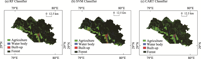
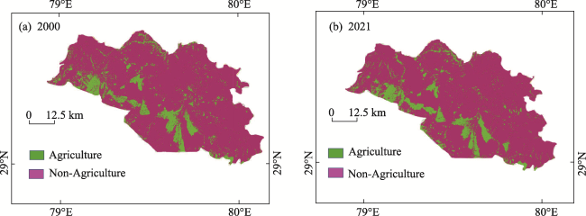
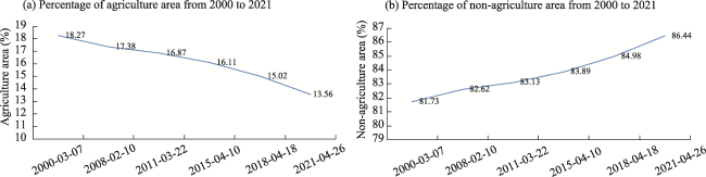
This study performs the time series analysis of agriculture land in the Nainital District of Uttarakhand, India. The study utilizes Landsat satellite images for the classification of agriculture and non-agriculture land over a time duration of 21 years (2000‒2021). Landsat 5, 7 and 8 satellites data have been used to classify the study area with Random Forest classifier. The Landsat satellite images are processed using the Google Earth Engine (GEE) platform. The selection of Random Forest classier has been based on a comparative analysis among Random Forest (RF), Support Vector Machines (SVM) and Classification and Regression Trees (CART). Overall accuracy, user accuracy and producer accuracy and Kappa coefficient has been evaluated to determine the best classifier for the study area. The overall accuracy for RF, SVM and CART for the year 2021 is 96.38%, 94.44% and 91.94% respectively. Similarly, the Kappa coefficient for RF, SVM and CART was 0.96, 0.89, 0.81 respectively. The classified images of Landsat in agriculture and non-agriculture area over a period of 21 years (2000-2021) shows a decrement of 4.71% in agriculture land which is quite significant. This study has also shown that the maximum decrease in agriculture area in last four years, i.e., from 2018 to 2021. This kind of study is very important for a developing country to access the change and take proper measure so that flora and fauna of the region can be maintained.

Cite this article

Saurabh PARGAIEN , Rishi PRAKASH , Ved Prakash DUBEY . Change of Agriculture Area over the Last 20 Years: A Case Study of Nainital District, Uttarakhand, India[J]. Journal of Resources and Ecology, 2023 , 14(5) : 983 -990 . DOI: 10.5814/j.issn.1674-764x.2023.05.009

1 Introduction

For a country, one of the most crucial aspects of its development circles around its capacity to produce food. For decades, agriculture has been associated with the production of essential food crops. The rate of urbanization at present is by-far the most superior aim of our civilization. In doing this, we are ignorantly diminishing our capacity for agriculture; especially in terms of land and fertility. As the amount of land will not be increasing in this era of urbanization and globalization, we will have to focus on making the most of what we have. Agriculture is a relevant activity for the global economy. India ranks second worldwide in farm output. India is an agrarian country and more than 60% of the population depends on agriculture for their livelihood. Agriculture Land is continuously decreasing and the demand is increasing. In India, agriculture has a huge impact on the national economy and most of the critical decisions are dependent on agricultural statistics.
Resource constraint is an issue which significantly affects any nation, and is even more profound in a developing economy like India. The burden on the limited resources is exacerbated by the huge population of the country making resource allocation even more difficult (Ratnaparkhi and Gawali, 2015; Abdi, 2020; Avashia et al., 2020; Fang et al., 2020). The inefficient use of limited available resources has led to unplanned development. Inefficient land use is a major cause of resource wastage. India is primarily an Agrarian economy with agricultural activities sustaining a major population. Therefore, it is imperative to utilize the available agricultural land such that maximum productivity can be achieved (Pal, 2005; Mallupattu and Sreenivasula, 2013; Maxwell et al., 2018; Nguyen et al., 2021; Tuvdendorj et al., 2022). The use of technology has been a boon for planned development models. With advancement in scientific research and technological aid, many time-consuming and effort intensive tasks can be done efficiently. The development of remote sensing technology and highly reliable imaging satellites has been providing accurate data covering almost every part of the Earth’s surface. Land cover data can be used for efficient monitoring and land management (Islam et al., 2018; Shivakumar and Rajashekararadhya, 2018). A careful assessment of land can be used to utilize the available land effectively and boost productivity without burdening the ecosystem. Land cover mapping aids in establishing the relationship between the environment and anthropogenic activities (Prakasam, 2010; Jensen and Cowen, 2011; Deorankar and Rohankar, 2020). Remote sensing satellite images can be used to examine the dynamic profile of land use land cover.
Nzhelele and Levhuvu catchments of the South Africa region were analysed using Landsat 8, Shuttle Radar Topography Mission (SRTM) Digital Elevation Model (DEM), Sentinel-1 and the GEE platform in 2017-2018. Ten land- cover classes using Random Forest classifier were analyzed with an overall accuracy of 76.43% (Zeng et al., 2020). The LULC change analysis of Tam Giang-Cau Hai of Southeast Asia was performed using LANDSAT, SPOT and ASTER remote sensing images. They were used to perform computer-aided visual interpretation resulting in an overall classification accuracy of 85% (Disperati and Virdis, 2015).
Surface reflectance data of Landsat 8 was analyzed to predict land cover maps of Mongolia. Eight different combination strategies using the Random Forest (RF) classifier were applied on the GEE platform with resulting overall accuracy over 84.31% (Phan et al., 2020). The impacts of LUCC on the environment of non-Amazonian South America was analyzed by considering the potential risks with respect to environment change (Salazar et al., 2015). MODIS data with 250 m resolution was used to map global cover land for the year 2001 (overall accuracy 74.93%) and 2010 (overall accuracy 75.17%) (Wang et al., 2015). In NE Asia, Landsat 8 (2014 image, 143 path/rows, 3290 scenes), improved Particle-Particle Particle-Mesh (PPPM) algorithm and Google Earth Engine (GEE) can successfully map paddy rice. The paddy rice map results in a producer (user) accuracy of 73% (92%) (Dong et al., 2016). The Area of Trasimeno Lake (central Italy), was analyzed in GEE by combining GLCM, SNIC, and ML Algorithms using Sentinel 2, Landsat 8, and Planet Scope data (Tassi and Vizzari, 2020). Normalized Difference Built-up Index (NDBI) was used to map urban parts from TM imagery automatically. The mapping accuracy was 92.6% (Zha et al., 2003). Klang Valley, Malaysia land cover monitoring using Landsat data (1988, 2003 and 2018) was performed. CART classifier was implemented on GEE platform and it results in the best accuracy (Wahap and Shafri, 2020). Using the RF classifier, the LULC map of 2018 was produced from C-band SAR data and compared with NRSC data. The confusion matrix displayed that the overall classification accuracy was 90.41% (Parida and Singh, 2021).
With the advancement of technology, the processing of high-volume data obtained from high resolution sensors is a very challenging task nowadays. Fast computing capacity is required for all high-resolution multi-source satellite sensors. GEE platform is providing efficient solutions for these challenging tasks. It is a cloud computing platform powered by Google’s cloud infrastructure. The time series analysis of earth resources is the best application of GEE (Gorelick et al., 2017). The availability of MODIS, Landsat, and Sentinel satellite data with multiple rich machine learning classifiers in GEE platform makes it very user friendly for the analysis of earth surface observation and pixel-based (PB) and object-oriented (OO) LULC classification in different aspects. The accessibility of internet application programming interface and computer resources makes it a good alternative to different data processing software. In GEE the high-volume data processing can be executed by writing simple script programming (Zhang et al., 2018; Gong et al., 2019; Singha et al., 2019; Tian et al., 2019). GEE platform is equipped with several machine learning algorithms such Random Forest (RF), Classification and Regression Trees (CART), Support Vector Machines (SVM).
In this study, the Nainital District of Uttarakhand State was selected to monitor the changes in the agriculture land area from 2000 to 2021. The major urban areas of Nainital District are Haldwani and Kathgodam. The development of the Kumaon region is associated with these areas. The last two decades geographical changes with respect to agriculture and non-agricultural areas can be analyzed to predict the future possibilities.

2 Material and methods

2.1 Study area and data source

Nainital District is located between 29°00'N-29°35'N latitudes and 78°50'E-79°50'E longitudes in the Uttarakhand state of India as shown in Fig. 1.
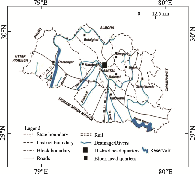
Fig. 1 Location map of Nainital District in the state of Uttarakhand, India
Uttarakhand state is located in the northern part of India. The maximum and minimum temperature of Nainital District is 27 ℃ and 10 ℃. The average annual temperature of Nainital District is 17.1 ℃. The annual rainfall is 1903 mm with major rainfall in august month. It is situated in the Bhabar region, the foothills of Kumaon Himalayas. Quartzite soil is generally found in this region. Wheat is cultivated on the maximum area in this region in winter. Rice, ragi, potato and tomato are summer crops. The other monsoon crops are maize and soyabean. Most of the study area is hilly terrain and its major land is covered by forest. The average elevation of Nainital District is 2084 m above sea level.
Landsat data has been utilized in this study. This study analysis the change in agriculture land over 20 years from 2000 to 2021 therefore, level 1 data of Landsat 7 and Landsat 8 data has been analyzed to determine the change statistics. Landsat 7 and Landsat 8 are equipped with TM, ETM+ and OLI sensors respectively. Google Earth Engine is an efficient platform to perform the classification of study area using different machine learning technique (Kelley et al., 2018; Teluguntla et al., 2018; Amani et al., 2019). Table 1 provide the details of the Landsat images used in the study.
Table 1 Details of landsat data used in the study
S.N. Acquisition date Sensor Spatial resolution Cloud cover
1 2021-04-26 Landsat 8 30 m Less than 10%
2 2020-03-22 Landsat 8 30 m Less than 10%
3 2019-05-07 Landsat 8 30 m Less than 10%
4 2018-04-18 Landsat 8 30 m Less than 10%
5 2017-02-10 Landsat 8 30 m Less than 10%
6 2016-05-14 Landsat 8 30 m Less than 10%
7 2015-04-10 Landsat 8 30 m Less than 10%
8 2014-01-10 Landsat 8 30 m Less than 10%
9 2013-03-13 Landsat 7 30 m Less than 10%
10 2012-01-20 Landsat 7 30 m Less than 10%
11 2011-03-22 Landsat 7 30 m Less than 10%
12 2010-03-19 Landsat 7 30 m Less than 10%
13 2009-03-16 Landsat 7 30 m Less than 10%
14 2008-02-10 Landsat 7 30 m Less than 10%
15 2007-05-14 Landsat 7 30 m Less than 10%
16 2006-02-04 Landsat 7 30 m Less than 10%
17 2005-04-06 Landsat 7 30 m Less than 10%
18 2004-02-15 Landsat 7 30 m Less than 10%
19 2003-02-12 Landsat 7 30 m Less than 10%
20 2002-01-01 Landsat 7 30 m Less than 10%
21 2001-01-21 Landsat 5 30 m Less than 10%
22 2000-03-07 Landsat 5 30 m Less than 10%

2.2 Classification

This paper analyses the change in agriculture area of Nainital District. The methodology adopted to achieve this objective involves the efficient classification of land cover in various classes with various machine learning techniques and determination of best technique for study area based on accuracy analysis. A flow chart of methodology is shown in Fig. 2.
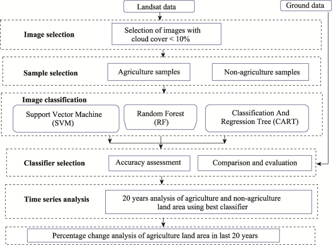
Fig. 2 The methodology used for LULC classification
The classification of Landsat images of the study area was carried out in four land cover classes which are agriculture, waterbody, built-up and forest. These were the most prominent land cover classes in the study area. Three different machine learning techniques have been applied on the Landsat images to classify it in aforementioned classes. These machine learning techniques are Random Forest (RF), Classification and Regression Trees (CART), Support Vector Machines (SVM). Most of the study area is hilly terrain therefore these three different machine learning techniques have been applied and further based on the accuracy assessment most efficient machine learning technique applicable for the study area has been selected. The selection of most suitable technique for study area to classify the land cover has been carried on Landsat image of year 2021. Once the suitable machine learning technique has been selected, it has been applied on the remaining Landsat images, i.e., images from the year 2000 to 2020. The selection of these three-classification technique is based on their applicability on satellite images by various researchers (Millard and Richardson, 2015; Li et al., 2016; Jin et al., 2018). Further, the approach utilised in classification of satellite images by these three machine learning techniques, i.e., RF, CART and SVM, are entirely different. The RF classifier is an ensemble classifier. It is a group of tree-structured classifiers in which different groups of decision trees are constructed. Here the number of decision trees are 100. The other parameters are the minimum leaf population and the bag fraction whose values is 1 and 0.5 respectively. A random vector as a parameter is selected by each decision tree which randomly selects the features of sample space. The subset of the sample data which is set as the training set is also selected randomly. This classifier splits each node using the best among a subset of predictors that is arbitrarily selected at that node. The final result is based on the majority voting. RF lessens decision tree overfitting and increases accuracy. It automates filling in data’s missing values. Because of a rule-based methodology data normalization is not required. To reduce overfitting, RF creates several trees to integrate their outputs, which need a lot of resources and computational power. As it integrates numerous decision trees to decide the class, training takes a lot of time. It also suffers from interpretability issues and is unable to establish the relative importance of each variable because of the ensemble of decision trees.
Whereas, in the CART algorithm the target variable is fixed. This algorithm is used to discover the class within which a target variable would most likely be categorised. In this, the value of outcome variable can be predicted based on other values. In this analysis for CART classifier, the value of smallest leaf population parameter is one and the largest node population parameter is null. On the basis of homogeneity of the data, classification tree separates the dataset. In a regression tree, a regression model is fit to the target variable using each of the independent variables. CART is transparent and simple to comprehend. It gives each decision in the problem specific input and output values so that every probability may be assessed. It is unstable and has a significant volatility and less effective when there are lots of uncorrelated variables in the problem.
RF and CART are decision tree-based approaches whereas SVM is basically a binary classifier that establishes a linear separating hyperplane to categorize data instances. The voting decision mechanism, linear function kernel type, null degree, and null gamma value are the parameters in the GEE environment for SVM, respectively. SVMs can be used for classification, regression, and clustering. SVMs can successfully deal with overfitting issues which are evident in high-dimensional spaces and are an appropriate choice for satellite image classification (Cánovas et al., 2017; Xia et al., 2017; Maxwell et al., 2019). SVM uses relatively less memory. Most used SVM algorithms contain the support vector regression, least squares support vector machine and successive projection algorithm-support vector machine. The limitation of SVM is the large data sets. When the target classes are overlapping and the data set includes more noise or when there are more training data samples than features for each data point, SVM does not perform very well.

2.3 Accuracy assessment

The assessment of classified image in different classes is made based on confusion matrix which provides the overall as well as class wise accuracies. A confusion matrix compares reference data and classification results relationship on a class-by-class basis. It helps in visualizing the performance of an algorithm based on class wise accuracy (i.e., user accuracy and producer accuracy) and overall accuracy. The overall accuracy in percentage specifies the proportion of correctly mapped sites out of all the reference sites. To calculate the overall accuracy, the sum of correctly classified pixels is divided by the sum of reference pixels. If the land cover classes are not evenly distributed, the overall accuracy should not be the only parameter to evaluate the performance of the classification technique. Class wise accuracy which are determined through user accuracy and producer accuracy provide the idea of performance of classification technique for each class. Further, Kappa coefficient which is based on KHAT statistics is good measure of accuracy for multiclass an imbalanced data set (Landis and Koch, 1977). Therefore, in this paper along with the overall accuracy, user accuracy and producer accuracy, Kappa coefficient has also been analyzed to determine the performance of three machine learning approaches which are RF, CART and SVM. Field surveys were conducted in the month of April because the date of Landsat image chosen for classification was April 26, 2021. Ground truth information is very much essential for training of satellite images for classification and then analysing the accuracies of classified image with different algorithms. Total 500 sample points were collected for agriculture category and total 710 sample points were considered for non-agriculture category. Out of 500 sample points that were considered for agriculture category, 350 were used as training data set and remaining 150 for analysing the accuracy. Similarly, in case of non-agriculture category, 510 and 200 points were considered for training and accuracy assessment respectively.

2.4 Time series analysis of agriculture land

The objective of this paper is to analyze the effect of urbanization on agriculture land in the study area. Therefore, the analysis has been categorized in agriculture and non-agriculture classes where non-agriculture classes include water bodies, urban and forest class. A time series analysis has been performed for last two decades, i.e., from the year 2000 to 2020. The selection of start year 2000 is based on the creation of new state Uttarakhand in 2000 in which study area lies. The creation of a new state led to the increased activities in state such as industrialization, tourism, government offices, schools and universities which led to the increase in urbanization in state. The time series analysis determines the percentage of agriculture area in different year and shows the decreasing behavior of agriculture area. RF algorithm has been used to determine the agriculture area in Landsat images of different years. The selection of RF is based on comparison analysis among RF, CART and SVM in which RF provide better result for the study area.

3 Result and analysis

Landsat image of 2021 of the study area has been utilised to classify the land cover in four classes using RF, CART and SVM. Figure 3a, 3b and 3c showed the classified Landsat image of the study area by using RF, SVM and CART, respectively. Agriculture has been shown in green colour, water bodies has been shown in blue colour, built-up area has been shown in red colour and forest area is in dark green colour. It is clearly evident from the classified image that most part of the study area is covered with forest. Table 2 showed PA, UA, OA and kappa coefficient for image classified with RF, SVM and CART, respectively. It can be clearly observed from the Table 2 that the highest overall accuracy has been obtained with RF classifier. The overall accuracy for RF, SVM and CART for the Landsat image of study area and of the year 2021 is 96.38%, 94.44% and 91.94% respectively. The overall accuracy of RF and SVM is comparable however, RF has performed better than SVM. Therefore, based on overall accuracy, RF may be selected to classify the Landsat images of study area. If we analyse the user and producer accuracies of these two classifiers for agriculture class, RF provide better results than SVM in both the cases. Further, Kappa coefficient is 0.96 in case of RF classifier whereas its value for SVM classifier is 0.89. Based on this analysis, RF has been chosen over SVM and CART to classify the Landsat images of study area spanning from the year 2000 to 2020.
Fig. 3 Classified outputs of Nainital District of 26 April 2021 based on different classifier
Table 2 Confusion matrix for the LULC map of 26 April 2021 using (a) RF Classifier; (b) SVM Classifier and (c) CART Classifier
Classes (a) RF Classifier (b) SVM Classifier (c) CART Classifier
Water
body
Forest Built-up Agriculture UA (%) Water
body
Forest Built-up Agriculture UA
(%)
Water
body
Forest Built-up Agriculture UA
(%)
Water body 54 2 1 3 90.00 59 0 1 0 98.33 53 0 3 4 88.33
Forest 0 59 0 1 98.33 0 54 0 6 90.00 1 52 0 7 86.67
Built-up 5 0 85 0 94.44 4 0 86 0 95.56 7 0 83 0 92.22
Agriculture 0 1 0 149 99.33 1 2 6 141 94.00 4 1 2 143 95.33
PA (%) 91.53 95.16 98.84 97.39 92.19 96.43 92.47 95.92 81.54 98.11 94.32 92.86
OA (%) 96.38 94.44 91.94
Kappa coefficient 0.96 0.89 0.81

Note: UA: The user accuracy; PA: Producer accuracy; OA: Overall accuracy.

Images of Landsat of study area were classified with RF classifier in agriculture, built-up, forest and water bodies. Further, built-up, forest, water bodies were considered as non-agriculture because the study in this paper concentrate towards the change in agriculture area over two decades (after the formation of Uttarakhand state in year 2000). Figure 5a and 5b show the classified images of study area of the year 2021 and 2000 in agriculture and non-agriculture classes, respectively. Figure 4a and 4b show the percentage of agriculture and non-agriculture in study area for different years, respectively. It can be clearly observed from the Fig. 5 that agriculture area has decreased by 4.71% and non-agriculture area has increased by 4.71% when a comparison is made from the year 2000 to the year 2021. An analysis from the year 2000 to 2008, 2008 to 2011, 2011 to 2015, 2015 to 2018 and 2018 to 2021 reveal that the agriculture area has decreased by 0.89%, 0.51%, 0.76%, 1.09% and 1.46%, respectively. The maximum change has been observed in the last four years, i.e., from 2018 to 2021. This fast change can be attributed to the fact development of urban area in Nainital District. The total area of Nainital District of Uttarakhand state is 4216 km2. As per the data of NRSC LULC Map of Uttarakhand State, in the year 2006 the total agriculture area of Nainital District was 19.25% and non-agriculture area was 80.75%. In the year 2015 the agriculture area was 17.95% and non-agriculture area was 82.05%. In these 10 years’ time span the agriculture area has decreased by 1.3% and non-agriculture area has increased by 1.3%. In our study, from 2008 to 2015 the change in agriculture area was 1.27%. There is a difference of 0.03% in the agriculture area between our study and NRSC study. This difference is due to number of years considered in the study. The NRSC study has taken 10-year difference whereas our study has considered a difference of 7 years. This comparison give strength to our study and validates our results.
Fig. 4 Agriculture and non-agriculture land area classification using random forest classifier (a) year 2000 (b) year 2021
Fig. 5 Percentage of land area using RF classifier analysis from 2000 to 2021 (a) agriculture area (b) non-agriculture area
Our results can also be justified with the following facts. In 2001 total population of Nainital District was 7.63 Lakh which increased to 9.55 Lakh in 2011. There is an increase of 25.16% in the population from 2001 to 2011. The estimated increase from 2011 to 2021 is 15.91 % and the predicted population for the year 2021 is 11.07 hundred thousand (Directorate of Census Operations in Uttarakhand, 2022). The major cities of Nainital District are Haldwani and Kathgodam. The population of these cities have increase around 16% from 2011 to 2021. If we analyse the increase in population of Nainital District in last two decades, i.e., from 2001-2021, it is 45%.
From 2001 to 2021, Nainital lost 9.39 kha of tree cover, equivalent to a 3.2% decrease in tree cover since 2000 (Global Forest Watch, 2021). The forest area is under the control of forest department of the state government and any activity in this class is strictly prohibited without the permission. The second class is waterbodies that is mainly river. There is a very less probability of encroachment in the river area. The increase in population needs residential and commercial area for their livelihood and activities. Most of the agriculture land is basically in the urban area. This is the main reason of the deduction in the agriculture area. A careful assessment of the results obtained can be very much helpful in developing infrastructure without degrading the balance of the ecosystem. This can prevent natural calamities like landslides which are frequent in the concerned area.

4 Conclusions

In this study, Landsat data along with RF classifier was used to extract the percentage change in agriculture area of Nainital District of Uttarakhand state in the last two decades, i.e., 2000 to 2021. The accuracy parameters for RF classifier, i.e., overall accuracy, Kappa coefficient, user and producer accuracy of agriculture area were higher than SVM and CART for the study area. Therefore, RF was used for the analysis of percentage change in agriculture and non-agriculture area of Nainital District. A decrement of 4.71% in agriculture area was observed during 2000-2021. During this period, the population of the study area grew by 45%. To validate the obtained results, a comparison has been made between our study and the study carried out by NRSC. A minor difference of 0.03% in agriculture area was observed between our study and NRSC study because our study considered 7 year of span and NRSC study considered 10 years of span. This comparison shows that the result obtained for the change in agriculture area between the years 2000 and 2021 is accurate. Further, it was observed that during same period study area has lost 9.39 kha of tree cover. This loss of tree belongs to the agriculture land as the forested area is monitored and governed by the state government and any activity is strictly prohibited in this area. The produced results in this paper led to the conclusion that the effect of population growth in the study area is causing the growth of the urban area which is mainly reducing the agriculture land. This study is very useful for government as well as non-government organization in planning and rehabilitation of growing population in the state.
[1]
Abdi A M. 2020. Land cover and land use classification performance of machine learning algorithms in a boreal landscape using Sentinel-2 data. GIScience & Remote Sensing, 57(1): 1-20.

[2]
Amani M, Mahdavi S, Afshar M, et al. 2019. Canadian wetland inventory using Google Earth Engine: The first map and preliminary results. Remote Sensing, 11(7): 842. DOI: 10.3390/rs11070842.

[3]
Avashia V, Parihar S, Garg A. 2020. Evaluation of classification techniques for land use change mapping of Indian cities. Journal of the Indian Society of Remote Sensing, 48(6): 877-908.

[4]
Cánovas-García F, Alonso-Sarría F, Gomariz-Castillo F, et al. 2017. Modification of the random forest algorithm to avoid statistical dependence problems when classifying remote sensing imagery. Computers & Geosciences, 103: 1-11.

[5]
Deorankar A V, Rohankar A A. 2020. An analytical approach for soil and land classification system using image processing. In: 2020 5th International Conference on Communication and Electronics Systems (ICCES) IEEE 1416-20. DOI: 10.1109/ICCES48766.2020.9137952.

[6]
Directorate of Census Operations in Uttarakhand. 2022. Nainital District: Population 2011-2022 data. https://www.census2011.co.in/census/district/584-nainital.Html. Viewed on 2022-09-20.

[7]
Disperati L, Virdis S G P. 2015. Assessment of land-use and land-cover changes from 1965 to 2014 in Tam Giang-Cau Hai Lagoon, central Vietnam. Applied Geography, 58: 48-64.

[8]
Dong J, Xiao X, Menarguez M A, et al. 2016. Mapping paddy rice planting area in northeastern Asia with Landsat 8 images, phenology-based algorithm and Google Earth Engine. Remote Sensing of Environment, 185: 142-154.

[9]
Fang P, Zhang X, Wei P, et al. 2020. The classification performance and mechanism of machine learning algorithms in winter wheat mapping using Sentinel-2 10-m resolution imagery. Applied Sciences, 10(15): 5075. DOI: 10.3390/app10155075.

[10]
Global Forest Watch. 2021. https://www.globalforestwatch.org/dashboards/country/IND. Viewed on 2021-10-20.

[11]
Gong P, Liu H, Zhang M, et al. 2019. Stable classification with limited sample: Transferring a 30-m resolution sample set collected in 2015 to mapping 10-m resolution global land cover in 2017. Science Bulletin, 64(6): 370-373.

[12]
Gorelick N, Hancher M, Dixon M, et al. 2017. Google Earth Engine: Planetary-scale geospatial analysis for everyone. Remote Sensing of Environment. 202: 18-27.

[13]
Islam K, Jashimuddin M, Nath B, 2018. Land use classification and change detection by using multi-temporal remotely sensed imagery: The case of Chunati wildlife sanctuary, Bangladesh. The Egyptian Journal of Remote Sensing and Space Science, 21(1): 37-47.

[14]
Jensen J R, Cowen D C. 2011. Remote sensing of urban/suburban infrastructure and socio-economic attributes,”In: Dodge M, Kitchin R, Perkins C(The map reader, 1st ed.,Eds.). John Wiley & Sons, Ltd: 153-163.

[15]
Jin Y, Liu X, Chen Y, et al. 2018. Land-cover mapping using Random Forest classification and incorporating NDVI time-series and texture: A case study of central Shandong. International Journal of Remote Sensing, 39(23): 8703-8723.

[16]
Kelley L C, Pitcher L, Bacon C. 2018. Using Google Earth Engine to map complex shade-grown coffee landscapes in Northern Nicaragua. Remote Sensing, 10(6): 952. DOI: 10.3390/rs10060952.

[17]
Landis J R, Koch G G. 1977. The measurement of observer agreement for categorical data. Biometrics, 33(1): 159-174.

[18]
Li X, Chen W, Cheng X, et al. 2016. A comparison of machine learning algorithms for mapping of complex surface-mined and agricultural landscapes using Ziyuan-3 stereo satellite imagery. Remote Sensing, 8(6): 514. DOI: 10.3390/rs8060514.

[19]
Mallupattu P K,Sreenivasula Reddy J R. 2013. Analysis of land use/land cover changes using remote sensing data and GIS at an urban area, Tirupati, India. The Scientific World Journal, 2013(6): 1-6.

[20]
Maxwell A E, Strager M P, Warner T A, et al. 2019. Large-area, high spatial resolution land cover mapping using Random Forests, GEOBIA, and NAIP orthophotography: Findings and recommendations. Remote Sensing, 11(12): 1409. DOI: 10.3390/rs11121409.

[21]
Maxwell A E, Warner T A, Fang F. 2018. Implementation of machine-learning classification in remote sensing: An applied review. International Journal of Remote Sensing, 39(9): 2784-2817.

[22]
Millard K, Richardson M. 2015. On the importance of training data sample selection in random forest image classification: A case study in peatland ecosystem mapping. Remote Sensing, 7(7): 8489-8515.

[23]
Nguyen-Van-Anh V, Hoang-Phi P, Nguyen-Kim T, et al. 2021. The influence of satellite image spatial resolution on mapping land use/land cover: A case study of Ho Chi Minh City, Vietnam. IOP Conference Series: Earth and Environmental Science, 652(1): 012002. DOI: 10.1088/1755-1315/652/1/012002.

[24]
Pal M. 2005. Random Forest classifier for remote sensing classification. International Journal of Remote Sensing, 26(1): 217-222. DOI: 10.108 0/01431160412331269698.

[25]
Parida B R, Singh S. 2021. Spatial mapping of winter wheat using C-band SAR (Sentinel-1A) data and yield prediction in Gorakhpur District, Uttar Pradesh (India). Spatial Science, 1-16. DOI: 10.1080/ 14498596.202 1.1896393.

[26]
Phan T N, Kuch V, Lehnert L W. 2020. Land cover classification using Google Earth Engine and Random Forest Classifier—The role of image composition. Remote Sensing, 12(15): 2411. DOI: 10.3390/rs12152411.

[27]
Prakasam C. 2010. Land use and land cover change detection through remote sensing approach: A case study of Kodaikanal Taluk, Tamilnadu. International Journal of Geomatics and Geosciences, 1: 46-55.

[28]
Ratnaparkhi N S, Gawali B W. 2015. Classification of land use and land cover using remotely sensed data for Parbhani City, Maharashtra, India. International Journal of Science and Research, 4(5): 269-272.

[29]
Salazar A, Baldi G, Hirota M, et al. 2015. Land use and land cover change impacts on the regional climate of non-Amazonian South America: A review. Global and Planetary Change, 128: 103-19. DOI: 10.1016/j. gloplacha.2015.02.009.

[30]
Shivakumar B R, Rajashekararadhya S V. 2018. Investigation on land cover mapping capability of Maximum Likelihood Classifier: A case study on North Canara, India. Procedia Computer Science, 143: 579-586.

[31]
Singha M, Dong J, Zhang G, et al. 2019. High resolution paddy rice maps in cloud-prone Bangladesh and Northeast India using Sentinel-1 data. Scientific Data, 6(1): 26. DOI: 10.1038/s41597-019-0036-3.

[32]
Tassi A, Vizzari M. 2020. Object-oriented LULC classification in Google Earth Engine combining SNIC, GLCM, and machine learning algorithms. Remote Sensing, 12(22): 3776. DOI: 10.3390/rs12223776.

[33]
Teluguntla P, Thenkabail P S, Oliphant A, et al. 2018. A 30-m landsat-derived cropland extent product of Australia and China using random forest machine learning algorithm on Google Earth Engine cloud computing platform. ISPRS Journal of Photogrammetry and Remote Sensing, 144: 325-340.

[34]
Tian F, Wu B, Zeng H, et al. 2019. Efficient identification of corn cultivation area with multitemporal synthetic aperture radar and optical images in the Google Earth Engine Cloud Platform. Remote Sensing, 11(6): 629. DOI: 10.3390/rs11060629.

[35]
Tuvdendorj B, Zeng H, Wu B, et al. 2022. Performance and the optimal integration of Sentinel-1/2 time-series features for crop classification in Northern Mongolia. Remote Sensing, 14(8): 1830. DOI: 10.3390/ rs14081830.

[36]
Wahap N A, Shafri H Z M. 2020. Utilization of Google Earth Engine (GEE) for land cover monitoring over Klang Valley, Malaysia. IOP Conference Series: Earth and Environmental Science, 540(1): 012003. DOI: 10.10 88/1755-1315/540/1/012003.

[37]
Wang J, Zhao Y, Li C. 2015. Mapping global land cover in 2001 and 2010 with spatial-temporal consistency at 250-m resolution. ISPRS Journal of Photogrammetry and Remote Sensing, 103: 38-47.

[38]
Xia J, Falco N, Benediktsson J A, et al. 2017. Hyperspectral image classification with rotation random forest via KPCA. IEEE Journal of Selected Topics in Applied Earth Observations and Remote Sensing, 10(4): 1601-1609.

[39]
Zeng H, Wu B, Wang S, et al. 2020. A synthesizing land-cover classification method based on Google Earth Engine: A case study in Nzhelele and Levhuvu Catchments, South Africa. Chinese Geographical Science, 30(3): 397-409.

[40]
Zha Y, Gao J, Ni S. 2003. Use of normalized difference built-up index in automatically mapping urban areas from TM imagery. International Journal of Remote Sensing, 24(3): 583-594.

[41]
Zhang X, Wu B, Ponce-Campos G, et al. 2018. Mapping up-to-date paddy rice extent at 10 m resolution in China through the integration of optical and synthetic aperture radar images. Remote Sensing, 10(8): 1200. DOI: 10.3390/rs10081200.

Outlines

/