Ecosystem and Ecological Function

Spatial and Temporal Evolution and Correlation Analysis of Landscape Ecological Risks and Ecosystem Service Values in the Jinsha River Basin

  • LIU Fenglian , * ,
  • YANG Lei ,
  • WANG Shu
Expand
  • Institute of Land & Resources and Sustainable Development, Yunnan University of Finance and Economics, Kunming 650221, China
*LIU Fenglian, E-mail: ;

Received date: 2022-12-11

  Accepted date: 2023-03-10

  Online published: 2023-08-02

Supported by

The Scientific Research Fund Project of Yunnan Education Department(2021J0592)

The Yunnan University of Finance and Economics Programme(2022D13)

The Graduate Student Innovation Fund Project of Yunnan University of Finance and Economics(2022YUFEYC098)

Abstract

Based on the land use data of 2000, 2010, and 2018, ArcGIS, Fragstas, and GeoDa software were used to assess the spatial and temporal evolution of ecosystem service value (ESV) and landscape ecological risk (LER) in the Jinsha River Basin from 2000 to 2018. Their relationship was subsequently examined using bivariate spatial autocorrelation and spatial regression models. The results indicate three important aspects of this system. (1) Between 2000 and 2018, the woodland, grassland, water area, and construction land rose, while the cultivated land and unused land declined, among which the decrease in unused land and the increase in construction land were more prominent. (2) From 2000 to 2018, the value of ecosystem services in the study area increased by 73.09 billion yuan, from 2018.89 billion yuan to 2091.98 billion yuan, while the overall landscape ecological risk index decreased from 0.01029 to 0.01021. The areas occupied by both low-risk and high-risk areas increased, indicating that the ecological environment in the region as a whole has been improving. However, there are still localized areas with deteriorating ecological conditions. (3) There is a positive spatial correlation between landscape ecological risk and ecosystem service values in the study area, demonstrating a high-risk-high-value clustering characteristic, and the landscape ecological risk has a positive effect on the value of all ecosystem services, particularly the value of the regulation services. The findings of this study can be used as a guide for reducing regional ecological risks, enhancing ecosystem services, and enhancing the quality of the ecological environment in the basin.

Cite this article

LIU Fenglian , YANG Lei , WANG Shu . Spatial and Temporal Evolution and Correlation Analysis of Landscape Ecological Risks and Ecosystem Service Values in the Jinsha River Basin[J]. Journal of Resources and Ecology, 2023 , 14(5) : 914 -927 . DOI: 10.5814/j.issn.1674-764x.2023.05.003

1 Introduction

Land use change has a significant effect on ecosystem services (Gong et al., 2021). It also impacts the quality of the ecological environment and directly or indirectly modifies the regional landscape pattern (Zhang et al., 2021). In addition, land use change is one of the primary sources of landscape ecological risk and a key driver of changes in the value of ecosystem services. An in-depth analysis of the coupled and coordinated relationship between landscape ecological risk and ecosystem service values can effectively correlate the ecological environment and human well-being (Zhu and Chen, 2022), which is essential for preventing regional landscape ecological risk, protecting and enhancing regional ecosystem functions, and promoting sustainable development of the social economy and the ecological environment (Li et al., 2021). The United Nations Millennium Ecosystem Assessment defines ecosystem services as the advantages humans obtain directly or indirectly from ecosystems, and it separates ecosystem services into four categories: supplying, supporting, regulating, and cultural (Reid et al., 2005). The value of ecosystem services is the monetary worth of ecosystem service functions, which helps humans understand the influences of their actions on the ecosystem and their well-being, thereby increasing awareness of the need for ecological conservation. Landscape ecological risk encompasses the likelihood and severity of damage caused by human activities, natural disasters, and other events that have detrimental effects on the structural functions of each ecosystem within the landscape (Hou et al., 2020). As an essential branch of ecological risk at the regional scale, landscape ecological risk mainly considers the perspective of landscape ecology, emphasizing the scale effect and spatial heterogeneity of the research object, and it is gradually becoming an essential tool for evaluating habitat quality and the characteristics of changes.
Ecological risk assessment and ecosystem service value assessment are crucial ecological and environmental assessment components that are strongly related to regional ecological safety assessment (Li and Gao, 2019). Specifically, research on ecosystem service value focuses on the impact of land use and landscape pattern changes on ESV, as well as the spatial and temporal evolution and drivers of ESV, along with the balance and coordination of ecosystem services. The research scale mainly involves province, city, county, and watershed; and research on landscape ecological risk focuses on landscape ecological risk assessment and spatiotemporal evolution characteristics, in addition to the construction of ecological network or ecological security patterns based on landscape ecological risk. However, with the gradual maturation of research on ESV and LER, the academic research on these topics began to move from independence to integration, mainly including three aspects. The first is incorporating ecosystem services into the ecological risk assessment framework and conducting an integrated assessment (Kang et al., 2018; Xing et al., 2020). The second includes integrating landscape ecological risks with ecosystem service values, categorizing the study area into different value-risk types, and implementing zoning control; locating high-priority conservation areas for natural heritage sites (Wang et al., 2022); bolstering urban ecological management to promote urban landscape planning and sustainable development (Su et al., 2012; Wu et al., 2022); and using coupled coordination degree models, multiple regression models, spatial autocorrelation analysis, and other methods, to discuss the correlations between landscape ecological risks and ecosystem service values (Zhang and Gao, 2016; Zhang et al., 2022a). Finally, some individual scholars analyze the impact of landscape pattern evolution on ecosystem service values from the perspective of landscape pattern changes (Zang et al., 2017; Chen and Huang, 2021).
Despite some forward movement in the study of the links between landscape ecological risk and ecosystem services value (Hu et al., 2021; Yang et al., 2021), there are still several open questions. 1) Few studies have investigated the link between landscape ecological risk and ecosystem service value; and those that have focused on this topic went no further than determining whether or not a correlation existed between ESV and LER, rather than exploring the extent to which landscape ecological risk affected the value of ecosystem services as a whole or any one individual service. Therefore, it is difficult to get to the heart of what connects them. 2) Current research focuses on economically- and populace-dense, highly developed, and utilized areas (Mo et al., 2017; Shen et al., 2021; Zhang et al., 2022b). In contrast, areas with sensitive and fragile ecological environments, complex topography, and crucial ecological conservation significance are given less attention. The Jinsha River Basin is located in the upper reaches of the Yangtze River, and it is a significant ecological security barrier in the upper reaches of the Yangtze River. Its ecosystem is fragile and belongs to the critical ecological function area with restricted development. Ecological problems such as soil erosion, rock desertification, and water pollution have occurred frequently in recent years. In light of these issues, this study takes the whole Jinsha River Basin as the study area and analyzes the spatial and temporal evolutionary characteristics of landscape ecological risk and ecosystem service value in the Jinsha River Basin based on land use change; and further determines the relationship between LER and ESV and the influence of LER on ESV, in order to develop suggested measures for improving ecosystem services and reducing ecological risk in the basin, as well as to provide a reference for ecological restoration and ecological security pattern construction in the basin.

2 Materials and methods

2.1 Study area

The Upper Yangtze is known as the Jinsha River. Its coordinates span 90°32'24"E to 104°57'00"E and 24°27'36"N to 35°46'48"N (Fig. 1). In western China, it passes through the provinces of Tibet, Qinghai, Sichuan, Yunnan, and Guizhou. The river basin is enormous, encompassing 473200 km2 (or 26% of the total area of the Yangtze River Basin). As a result of the river delta topography in the Hengduan Mountains, the site is long and narrow with a north-south orientation. It includes a portion of the Tibetan Plateau, the northern Yunnan Plateau, the Sichuan Basin, and the Hengduan Mountains. The basin’s climate is distinct, with distinct vertical distribution characteristics, such as plateau mountain climate, dry-hot valley climate, and other climate types. The basin has abundant water resources, primarily natural precipitation, with an average annual precipitation of about 710 mm. Furthermore, the Jinsha River Basin is home to various nationally rare and endangered animals and plants. It is the area with the greatest wealth of biological communities in Eurasia, providing migration routes and refuges for many biological species from south to north.
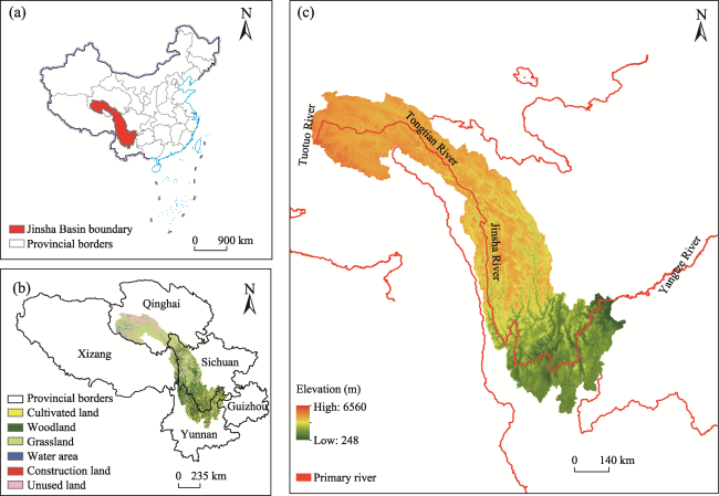
Fig. 1 Location of the Jinsha River Basin

2.2 Data sources and methods

2.2.1 Data source

The land use raster data used in this study were obtained from the Chinese Academy of Sciences Resource and Environment Science and Data Center (http://www.resdc.cn), where the land use data from 2000 and 2010 were inter preted using Landsat TM/ETM remote sensing images, and the land use data from 2018 were interpreted using Landsat 8 remote sensing imagery, which has a spatial resolution of 30 m. The interpretation accuracy was greater than 90%, and the land use types were classified as cultivated land, woodland, grassland, water area, construction land, and unused land. This dataset is currently China’s most accurate land use remote sensing monitoring data product (Li et al., 2018; Zhang et al., 2020). DEM data were obtained from the geospatial data cloud platform (http://www.gscloud.cn), and data on average grain production in the Jinsha River basin’s five provinces and nationally were obtained from the China Agricultural Yearbook.
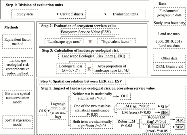
Fig. 2 Technical flow chart

2.2.2 Evaluation of ecosystem services value

Based on the equivalency factor approach presented by Costanza et al. (1997), Xie et al. (2015) calculated the value of ecosystem services in China for one standard equivalence factor at 3406.5 yuan ha-1. Adjusting that figure by a correction factor of 0.86 for the study area acquired from the grain production in the Jinsha River basin and the national grain production in that year, yields a final economic value of ecosystem services per unit area in the Jinsha River Basin of 2929.59 yuan ha-1. Ecosystem services can be quantified with the following formula (Lin et al., 2013):
$ESV\text{=}\underset{k\text{=1}}{\overset{n}{\mathop \sum }}\,{{S}_{k}}\times V{{C}_{k}}$
$ES{{V}_{f}}\text{=}\underset{k\text{=1}}{\overset{n}{\mathop \sum }}\,{{S}_{k}}\times V{{C}_{kf}}$
where ESV is the overall economic value of ecosystem services in the Jinsha River Basin, and ESVf is the economic value of each unique ecosystem service in the research region; n indicates the number of landscape types involved in this study; k is a landscape type and Sk is the area of that type; f denotes the f-th individual ecosystem service; and VCk and VCkf are the ecosystem service value (ESV) coefficient for that landscape type and the ESV coefficient for that service, respectively.
The values of ecosystem services per unit area of distinct landscape ecosystems in the Jinsha River basin were evaluated using the fundamental equivalence table of the functional value of ecosystem services per unit area presented by Xie et al. (2015), along with the landscape types of the basin, while taking into account the detrimental influence of the construction land on ecosystem services due to the dramatic amount of human activity (Yang et al., 2018) (Table 1).
Table 1 Ecosystem service values per unit area of different landscape ecosystems in Jinsha River Basin from 2000 to 2018 (Unit: yuan ha-1)
Primary classification Secondary classification Cultivated land Woodland Grassland Water area Construction land Unused land
Supply services Food production 2490.15 849.58 539.04 2343.67 0.00 8.79
Raw material production 1171.84 1933.53 799.78 673.81 -22001.22 26.37
Water supply 58.59 996.06 439.44 24286.30 -7089.61 17.58
Regulating services Gas regulation 1962.83 6357.21 2786.04 2255.78 0.00 137.69
Climate regulation 1054.65 19042.34 7370.85 6708.76 -7206.79 87.89
Purify the environment 292.96 5654.11 2437.42 16259.22 0.00 477.52
Hydrological regulation 790.99 13886.26 5393.38 299521.28 58.59 246.09
Support services Soil conservation 3017.48 7763.41 3395.39 2724.52 0.00 155.27
Maintain nutrient cycling 351.55 585.92 269.52 205.07 996.06 8.79
Biodiversity 380.85 7060.31 3096.58 7470.45 29.30 146.48
Cultural services Aesthetic landscapes 175.78 3105.37 1368.12 5536.93 58.59 64.45

2.2.3 Evaluation of landscape ecological risk

Firstly, the Fragstats software was used to calculate the landscape fragmentation (Ci), landscape separation (Si), and landscape dominance indexes (Di). Next, these three indexes were given weights of 0.5, 0.3, and 0.2, and the landscape disturbance index (Ui) was then derived via the weighted summation. By weighting and summing, the landscape disturbance index was created.
Secondly, in the sequence of decreasing vulnerability: developed land 1, forest land 2, grassland 3, cultivated land 4, water area 5, unused land 6, the types were normalized to obtain the landscape vulnerability index (Ei) values of the various landscape types.
Thirdly, we multiplied the landscape disturbance index (Ui) by the landscape vulnerability index (Ei) to obtain the landscape loss index (Ri).
Finally, the landscape ecological risk index (LERI) was calculated using the landscape vulnerability index and the area proportions of the landscape components. The following is an expression of that formula (Wang et al., 2021):
$LERI\text{=}\underset{i\text{=1}}{\overset{n}{\mathop \sum }}\,\frac{{{A}_{ki}}}{{{A}_{k}}}\times {{R}_{i}}$
where LERI is the Landscape Ecological Risk Index, the greater the value, the greater the regional landscape ecological risk; i denotes the i-th type of landscape; n denotes the total number of landscape types; and Aki is the area of class i landscape in the k-th risk community; Ak is the total area of class i landscape; Ri is the landscape loss index.

2.2.4 Bivariate Spatial Autocorrelation Model

The objective of spatial autocorrelation analysis is to determine whether a variable is spatially correlated and the strength of that connection. It is used to characterize the spatial distribution characteristics of a variable and the extent of its influence on surrounding units. The analysis of spatial autocorrelation encompasses both global and local spatial autocorrelation (Fang et al., 2015). Some researchers have constructed bivariate global spatial autocorrelation and local spatial autocorrelation in order to investigate the spatial correlation between many variables (Wartenberg, 1985). This provides a straightforward method for examining how landscape ecological risks affect ecosystem service value. This study examined spatial autocorrelation analysis using GeoDa1.14 software.
Bivariate Global Moran’s I was calculated as follows (Shen and Zeng, 2021):
$I\text{=}\frac{\sum\limits_{i=1}^{n}{\sum\limits_{j=1}^{n}{{{W}_{ij}}({{x}_{i}}\text{--}\bar{x})({{y}_{j}}-\bar{y})}}}{{{S}^{\text{2}}}\sum\limits_{i=1}^{n}{\sum\limits_{j=1}^{n}{{{W}_{ij}}}}}$
where I represents the bivariate global spatial autocorrelation index and n represents the number of spatial units; Wij represents the spatial weight matrix; xi and yi are the observed values of independent variables and dependent variables in spatial units i and j, respectively; $\bar{x}$ and $\bar{y}$ are the average values of x and y, respectively; and S2 is the sample variance.
Bivariate Local Moran’s I was calculated as follows (Shen and Zeng, 2021):
${{I}_{i}}\text{=}{{z}_{i}}\underset{j\text{=1}}{\overset{n}{\mathop \sum }}\,{{w}_{ij}}{{z}_{j}}$
where Ii is the bivariate local spatial autocorrelation index; zi and zj are the normalized values of the observed variances of the spatial units i and j; n represents the number of spatial units; and wij represents the spatial weight matrix.

2.2.5 Spatial Regression Model

When we assess a set of data for analysis, we usually start by using the ordinary least square method to determine if the data pass the significance test. This allows us to determine whether there is any spatial correlation between variables, or whether there is similarity or heterogeneity between the explained variables and their adjacent spatial units. Then, using the Lagrange Multiplier (LM) test of the OLS model, we assess whether the P values of LM (lag) and LM (error) are statistically significant in order to select a model. This process may involve the following scenarios: 1) If neither of the tests is statistically significant, the OLS model is used for the regression analysis; 2) If the LM (lag) test is statistically significant but the LM (error) test is not, or the significance levels are such that LM (lag) > LM (error), the SLM model is used, and vice versa; and 3) A robust level test is required if all of them are statistically significant. At this point, if the significance level is robust, i.e., LM (lag) > robust LM (error), then the SLM model is preferable; otherwise, the SEM model is appropriate. The following are the calculation methods for the two spatial regression models.
(1) Spatial Lag Model
$y\text{=}\rho {{W}_{y}}\text{+}X\beta \text{+}\varepsilon $
where y is the dependent variable; $\rho$ is the spatial autocorrelation parameter; Wy is the spatial lag vector of the dependent variable; X is an independent variable; $\beta$ is the spatial regression coefficient of the independent variable, and is the random error term (Anselin, 2002).
(2) Spatial Error Model
$\text{ }\!\!~\!\!\text{ }y\text{=}X\beta \text{+}\varepsilon \varepsilon \text{=}\lambda {{W}_{\varepsilon }}\text{+}\mu \mu \text{ }\!\!\tilde{\ }\!\!\text{ }N(\text{0, }{{\sigma }^{\text{2}}})$
where y is the dependent variable; X is an independent variable; $\beta ~$ is an estimated parameter; $\varepsilon $ is the vector of error terms; λ is the spatial autoregressive coefficient of the error term; ${{W}_{\varepsilon }}$ is the spatial lag vector of the spatial error term; and $\mu $ is an uncorrelated error term with zero expectation and homoscedasticity (Wu and Li, 2018).

3 Results

3.1 Analysis of land use change

The Jinsha River Basin is in western China and part of the upper reaches of the Yangtze River Basin. Because of its narrow and diverse topography, the population density and land development intensity vary widely within the basin. The Yunnan-Sichuan section is characterized by a large population, frequent human activity, and extensive changes in land cover use. Because the climate of the Qinghai-Tibet Plateau is dry and cold and the topography is mountainous, neither of which are conducive to the growth of trees, grassland is the predominant land use type in the basin, accounting for roughly half of its total area (Table 2). The forest land and cultivated land are primarily dispersed in Sichuan and Yunnan in the lower portions of the river basin, where the temperature is quite warm and humid, and hence conducive to agriculture. Due to the limited natural environment in Qinghai, Tibet, it is difficult to cultivate a variety of grains, and grazing is the primary source of income. In addition, the vast distribution of alpine, anoxic, and frozen soil makes it impossible to develop and use the land in the upper reaches of the Jinsha River Basin, increasing the amount of unused area.
Table 2 Areas of various landscape types in Jinsha River Basin from 2000 to 2018
Landscape type 2000 2010 2018 2000-2018
Area (km2) Proportion (%) Area (km2) Proportion (%) Area (km2) Proportion (%) Area (km2) Proportion (%)
Cultivated land 32555.69 6.88 32734.70 6.92 32208.48 6.81 -347.20 -1.07
Woodland 139681.69 29.52 144953.64 30.63 144756.33 30.59 5074.63 3.63
Grassland 237002.86 50.09 240607.15 50.85 240147.70 50.75 3144.84 1.33
Water area 10234.31 2.16 10766.50 2.28 11225.82 2.37 991.51 9.69
Construction land 992.74 0.21 1515.56 0.32 2269.61 0.48 1276.87 128.62
Unused land 52732.72 11.14 42622.45 9.01 42592.06 9.00 -10140.66 -19.23
Total area 473200.00 100.00 473200.00 100.00 473200.00 100.00 0 0
From 2000 to 2018, the land use pattern in the Jinsha River Basin clearly changed, and the unused land decreased dramatically, with a total decrease of 10140.66 km2, accounting for 19.23% of the full unused land area. The quantity of farmed land increased before declining. From 2000 to 2010, the amount of cultivated land increased somewhat, however, the amount of cultivated land decreased from 2010 to 2018 by 347.20 km2. The areas of the other four land use groups have all expanded, especially the amount of construction land which more than doubled between 2000 and 2018. The additional construction land is primarily distributed in Panzhihua City and Liangshan Prefecture in southern Sichuan Province downstream of the basin, as well as in Diqing Prefecture, Lijiang City, Chuxiong Prefecture, Kunming City, and Zhaotong City in northern Yunnan Province, with Kunming City experiencing the greatest increase. In addition, forest land and grassland rose during the research period by 5074.63 km2 and 3144.84 km2, respectively, mainly due to the 1999 implementation of the project to restore cropland to forest and grassland in the Jinsha River Basin. Since 2000, Yunnan Province has implemented a trial project to return cropland to forest and grassland, focusing on the Jinsha River Basin. This has significantly improved the natural environment of the region while increasing the forest and green space coverage.

3.2 Analysis of ecosystem service value

The value of ecosystem services is an essential indicator for measuring the ecosystem service supply capacity (De Groot et al., 2012). Regarding the value of ecosystem services of different land use types, the total value of ecosystem services in the Jinsha River basin has been increasing, with a total increase of 73.09 billion yuan from 2000-2018 (Table 3). During the study period, forest land contributed the most to the value of ecosystem services, accounting for more than 46% of the total ESV, with an increase of 34.12 billion yuan. The value of ecosystem services offered by grassland is second only to that of forests, and the trend of change is identical to that of forest ESV. The water area is the third largest land use type contributing to the provision of ecosystem service value in the Jinsha River Basin, and its contribution to the total ecosystem service value is growing over time. The ESV supply capacities of farmed land and unused land are relatively low. Building land is a type of land that is required by the environment. Due to the interference from human activities and the exploitation of natural resources, its positive influence on ecosystem services is significantly less than its negative effect; therefore, it will offset the contributions of other land types to ecosystem services. Recent years have seen substantial growth in construction land, so the ESV of construction land should not be overlooked when estimating the ESV of the study region.
Table 3 Changes of land ESV in Jinsha River Basin from 2000 to 2018
Landscape type 2000 2010 2018 2000-2018
ESV (108 yuan) Proportion (%) ESV (108 yuan) Proportion (%) ESV (108 yuan) Proportion (%) ESV (108 yuan) Proportion (%)
Cultivated land 382.45 1.89 384.56 1.85 378.37 1.81 -4.08 -1.07
Woodland 9391.37 46.52 9745.83 46.83 9732.56 46.52 341.19 3.63
Grassland 6611.33 32.75 6711.87 32.25 6699.05 32.02 87.73 1.33
Water area 3766.08 18.65 3961.92 19.04 4130.94 19.75 364.86 9.69
Construction land -34.90 -0.17 -53.28 -0.26 -79.79 -0.38 -44.89 128.62
Unused land 72.61 0.36 58.69 0.28 58.65 0.28 -13.96 -19.23
Total ESV 20188.94 100.00 20809.58 100.00 20919.79 100.00 730.85 3.62
Regarding the value of individual ecosystem services (Table 4), regulation services have a comparative advantage of 69.72%, whereas support, provisioning, and cultural services are relatively poor. Eleven secondary ecosystem services had higher values for climate management and hydrological regulation, but lower values for food production, raw material production, and water supply. In terms of changes in the ESV provided by secondary ecosystem service types, the ecosystem service function of raw material production declined, and its ecosystem service value decreased by a total of 1.58 billion yuan. Between 2000 and 2018, hydro-logical regulation, climate regulation, gas regulation, biodiversity, soil conservation, and purifying the environment had greater growth in their ecosystem service values, with hydrological regulation experiencing the most extraordinary ESV growth. Changes in the ESV values of food production and maintaining nutrient cycling were insignificant.
Table 4 The ESV values of each ecosystem service in Jinsha River Basin from 2000 to 2018
Primary
classification
Secondary classification 2000 2010 2018 2000-2018
ESV
(×108 yuan)
Proportion
(%)
ESV
(×108 yuan)
Proportion
(%)
ESV
(×108 yuan)
Proportion
(%)
ESV
(×108 yuan)
Proportion
(%)
Supply
services
(6.48%)
Food production 351.94 1.74 359.97 1.73 359.32 1.72 7.38 2.10
Raw material production 484.22 2.40 486.10 2.34 468.45 2.24 -15.77 -3.26
Water supply 487.63 2.42 503.52 2.42 508.90 2.43 21.27 4.36
Regulating
services
(69.72%)
Gas regulation 1642.53 8.14 1686.25 8.10 1683.71 8.05 41.18 2.51
Climate regulation 4507.25 22.33 4633.31 22.27 4623.26 22.10 116.01 2.57
Purifying the environment 1568.57 7.77 1611.04 7.74 1616.11 7.73 47.53 3.03
Hydrological regulation 6322.08 31.31 6571.82 31.58 6703.79 32.05 381.71 6.04
Support
services
(19.73%)
Soil conservation 2023.43 10.02 2077.02 9.98 2073.59 9.91 50.15 2.48
Maintaining nutrient cycling 160.72 0.80 165.38 0.79 165.80 0.79 5.08 3.16
Biodiversity 1816.70 9.00 1867.66 8.98 1868.09 8.93 51.39 2.83
Cultural services
(4.07%)
Aesthetic landscapes 823.86 4.08 847.52 4.07 848.77 4.06 24.91 3.02
The study region was divided into 20 km by 20 km grids, yielding 1355 evaluation units, and the ESV of each grid was calculated based on the areas of various land use types and the values of ecosystem services per unit area. The spatial depiction of ESV via Kriging interpolation and the superposition of administrative-territorial entity data can illustrate the distribution of the various ESV levels. Five categories were assigned as low value region (0.5314-1.26946 billion yuan), sub-low value region (1.26947-1.80998 billion yuan), medium value region (1.80999-2.53968 billion yuan), sub-high value region (2.53969-3.78288 billion yuan), and high value region (3.78289-7.1845 billion yuan). The High value region and the sub-high value area are mostly spread out at both ends of the basin (Fig. 3), the medium value area is distributed in the middle and lower reaches, and the low value area and the sub-low value area are distributed in the middle and upper reaches. The areas that have high and sub-high values include: Geermu, northwestern Litang County, central Yajiang County, southern Xiangcheng County, northern Lijiang Naxi Autonomous County, at the junction of Yongsheng County, Dayao County, Yongren County, and Huaping County, and at the junction of Western Luquan Yi and Miao Autonomous County, Xishan District, Jinning District, and Chenggong District.
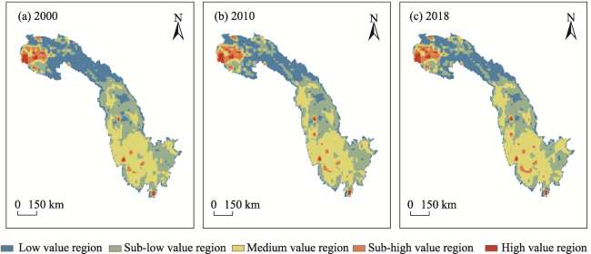
Fig. 3 Spatial distribution of ESV in Jinsha River Basin from 2000 to 2018
The data in Table 5 show the changes in the areas and proportions of areas which represent different levels of ecosystem service values in the Jinsha River Basin during 2000-2018. The areas occupied by the sub-low value area, the medium value area, and the low value area accounted for more than 93% of the total area of the study area, while the sub-highe value and high value areas were relatively few, accounting for less than 7% of the total area of the study area. Among them, the areas in other ecosystem service value classes increased from 2000 to 2010, except for thedecrease in the low value areas, indicating that the ecosystem service function had improved and the ecological environment became better during this period. The low, medium, and high value areas of ESV increased from 2010 to 2018, whereas the sub-low and high value areas decreased. These trends imply that while the general level of the ecological environment improved over this period, the ecological environment deteriorated in specific regions, which requires the attention of the relevant departments. From 2000 to 2018, the areas occupied by low value and sub-low value areas fell by 16916.98 km2 and 2177.19 km2, respectively, whereas high ecosystem service value areas increased dramatically. The main reason for the overall improvement is that the state has consistently carried out Yangtze River Basin protection in recent years, which included adhering to green development and pollution prevention, implementing normalized ecological restoration, afforestation, and increased forest coverage, and effectively curbing soil erosion, thus continuously improving biodiversity and the overall ecological environment.
Table 5 Areas and proportions of the different ESV classes
ESV of different grades 2000 2010 2018 2000-2018
Area (km2) Proportion (%) Area (km2) Proportion (%) Area (km2) Proportion (%) Area (km2) Proportion (%)
Low value region 133033.54 28.11 115065.5 24.32 116116.56 24.54 -16916.98 -12.72
Sub-low value region 165541.17 34.98 170871.52 36.11 163363.99 34.52 -2177.19 -1.32
Medium value region 147598.16 31.19 157583.18 33.30 161987.6 34.23 14389.44 9.75
Sub-high value region 21121.2 4.46 23248.34 4.91 25350.45 5.36 4229.25 20.02
High value region 5905.93 1.25 6431.46 1.36 6381.41 1.35 475.48 8.05

3.3 Analysis of landscape ecological risk

The landscape index, as a spatial analysis approach, may reflect the landscape pattern structure and spatial configuration characteristics, and efficiently tie the landscape pattern to ecological processes. Systematic investigation of the landscape index changes of different landscape types in the study area is critical for comprehending the regional landscape pattern changes. According to the landscape index (Fig. 4a), the landscape fragmentation of construction land was the highest among the six landscape types from 2000 to 2018, but the fragmentation gradually decreased with time. The fragmentation degree of water and cultivated land is second only to that of construction land, but the trend of change is the opposite of that of construction land. The degrees of fragmentation of woodland, grassland, and unused land are low, indicating that these landscape types are reasonably concentrated in space. Construction land, water area, and cultivated land are the landscape types with the highest degrees of landscape separation, and their patterns of change are essentially consistent with their degrees of fragmentation. The landscape dominance index indicates grassland, forest, cultivated land, unused land, water area, and building land in order of size, and this sequence is strongly related to the landscape type size. The landscape disturbance degree of the building land is the highest, indicating that human activities have seriously affected the terrain. Overall, the landscape loss degrees of water area and building land are substantial during the study period, but their loss degrees gradually diminished. It is worth mentioning that the landscape loss of cultivated land became more and more severe as time passed.
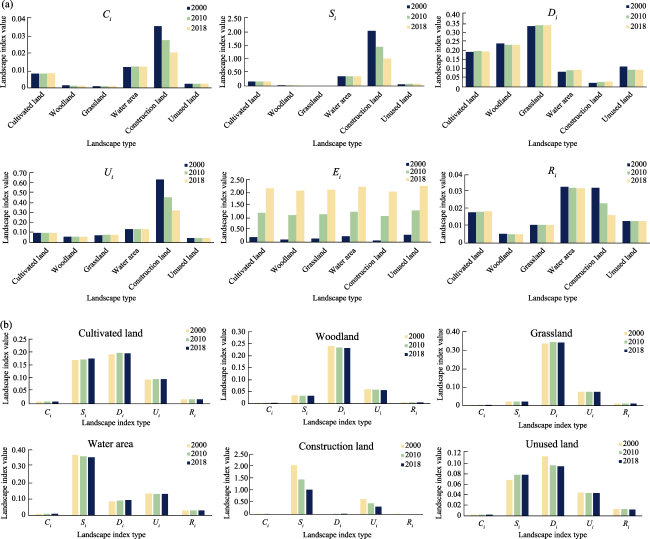
Fig. 4 Changes in the landscape index values of different landscape types in Jinsha River Basin from 2000 to 2018
From the perspective of landscape types (Fig. 4b), the fragmentation of cultivated land in the study area is becoming more serious. The degrees of separation, disturbance and loss are gradually increasing, which indicates that the cultivated land landscape is seriously affected by the external environment, and the ecological risk is rising progressively. This phenomenon suggests that the acquired land landscape is seriously affected by the external environment, and the ecological threat is gradually growing. Compared to other landscape indexes, the dominance of forest land is greater but declining. However, fragmentation and loss are relatively small, indicating that the forest land ecosystem is reasonably stable and its ecological loss tends to be reduced. The changes in the characteristics of the landscape index of grassland are similar to those of woodland. The landscape separation degree of the water area is relatively prominent, but it decreases with time. The reason for this decrease is that the spatial distribution of the water area is scattered, but the increase of water area reduces the separation degree. Among the landscape types, landscape fragmentation, separation, and disturbance of construction land are the most prominent. The values of the three landscape indexes gradually decrease with time, indicating that construction land aggregation is poor. Still, the stability and risk resistance are steadily improving. The extent of unused land has dropped significantly, and the degrees of fragmentation and separation have increased between 2000 and 2010 and they declined between 2010 and 2018, with disturbance and loss regularly declining. Overall, the level of landscape ecological security of unused land has been improving.
The values for the entire landscape ecological hazard of the Jinsha River Basin were 0.01029, 0.01024, and 0.01021 in 2000, 2010, and 2018, respectively, indicating that the ecological environment of the research region was constantlyimproving and the health status of the ecosystem was gradually improving. The ecological risk of a watershed landscape can be shown in space using Kriging interpolation. The ecological danger of a watershed landscape was graded into five levels using the natural discontinuity approach. The levels are as follows: low-risk region (0.0036-0.0463), sub-low-risk region (0.0463-0.0662), medium-risk region (0.0662-0.0844), and high-risk region (0.0844-0.1042). The high-risk and sub-high-risk areas are primarily located in the basin's head and tail areas and the middle Jinsha River main stream flowing area (Fig. 5). Specifically, the majority of the high-risk regions occurred in Geermu City, Qinghai Province, Xichang City, Panzhihua City, Yibin City, Sichuan Province, Kunming City, and Zhaotong City, Yunnan Province. From the perspective of county-level administrative regions, they included Geermu City in Qinghai; Mianning, Xide, Zhaojue, Xichang, Dechang, Puge, Butuo, Jinyang, Yanbian, Miyi, ningnan county, Huili, Huidong, Panzhihua, pingshan county, Shuifu and Suijiang in Sichuan; Dongchuan, Chuxiong, Mouding, Nanhua, Xishan, Jinning, Malong and Zhaotong in Yunnan. The moderate and low danger zones are widely dispersed throughout the center of the basin. From 2000 to 2018, the areas occupied by low-risk, sub-high-risk, and high-risk areas in the basin grew (Table 6), by 17692.76 km2, 4054.07 km2, and 8984.02 km2, respectively, whereas the regions of sub-low-risk and medium-risk areas decreased. These results indicate that the ecological environment as a whole has been continually improving. However, the landscape ecological dangers are increasing in certain regions.
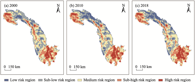
Fig. 5 Spatial distribution of landscape ecological risk in Jinsha River Basin from 2000 to 2018
Table 6 Area distribution of the different LER classes
Level of risk 2000 2010 2018 2000-2018
Area (km2) Proportion (%) Area (km2) Proportion (%) Area (km2) Proportion (%) Area (km2) Proportion (%)
Low-risk region 41566.72 8.78 59810.04 12.64 59259.48 12.52 17692.76 42.56
Sub-low-risk region 134735.25 28.47 121396.86 25.65 115566.01 24.42 -19169.24 -14.23
Medium-risk region 141692.23 29.94 134960.47 28.52 130130.63 27.50 -11561.61 -8.16
Sub-high-risk region 109409.83 23.12 108634.05 22.96 113463.90 23.98 4054.07 3.71
High-risk region 45795.97 9.68 48398.58 10.23 54779.99 11.58 8984.02 19.62

3.4 Relationships between landscape ecological risk and ecosystem service values

3.4.1 Spatial correlation analysis of LER and ESV

We set up a spatial weight matrix in GeoDa software to calculate the spatial correlation between landscape ecological risk and ecosystem service values in the Jinsha River Basin in 2000, 2010 and 2018. A Moran’s I scatter plot was obtained as shown in Fig. 6. The Global Moran’s I values in 2000, 2010 and 2018 were 0.310, 0.312, and 0.318, respectively, indicating a positive spatial correlation between LER and ESV. The correlation between LER and ESV increased gradually with time during the study period.
The clustering diagram of bivariate local spatial autocorrelation in Fig. 7 shows that the clustering relationship contains five types. Among them, the high-risk-high value area involves Geermu City in Qinghai Province in the upper part of the watershed, Xichang and Panzhihua City in Sichuan Province in the lower leg, and a part of Lijiang and Kunming City in Yunnan Province. The high-risk-low value areas are distributed around the high-value-high-risk regions and have a lower capacity to provide ecosystem services but a higher potential ecological risk. The low-risk-high-value areas are mainly distributed in Zhongdian County, northwestern Xichang City, and northwest Chuxiong City. The low-risk-low value parts are distributed primarily in the areas on both sides of the mainstream of Jinsha River, and mainly concentrated in Zhiduo County of Yushu Prefecture, Qinghai Province, and Kangding County of Ganzi Prefecture, Sichuan Province.
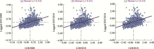
Fig. 6 Moran’s I scatter plot of Jinsha River Basin from 2000 to 2018
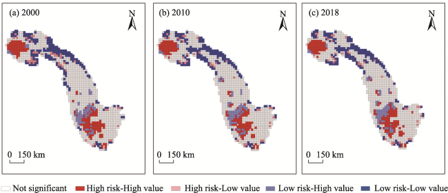
Fig. 7 LISA cluster map of Jinsha River Basin from 2000 to 2018

3.4.2 Impact of landscape ecological risk on ecosystem service value

By analyzing the spatial autocorrelation of landscape ecological risk and ecosystem service value, it is evident that LER and ESV have a robust spatial association. The degree of their influence is uncertain, but the alteration of landscape structure will affect the services and functions of the ecosystem, and the deterioration of the ecosystem will exacerbate the ecological risk of the regional landscape (Xing et al., 2020). To further investigate the impact of LER on ESV, we employed a spatial regression model. Using the landscape ecological risk index values of each risk assessment unit in 2000, 2010, and 2018 as independent variables and the total amount of ESV, supply service value, regulating service value, support service value, and cultural service value in the risk assessment unit in the same period as dependent variables, the spatial regression analysis was performed one-by-one to explore the extent of the influence of LER on Total of ESV and the values of the individual ecosystem services.
As a first step, the Moran test was used to determine the existence of a spatial correlation between landscape ecological risk and ecosystem service value, which was followed by ordinary least squares regression, and suitable spatial econometric models were then chosen based on the LM test and robustness test. According to the test results, the total of ESV, supply services value, regulating services value, and support services value data in 2000 are applicable to the spatial lag model, while the rest of the data are applicable to the spatial error model, and all data pass the significance test at the 1% level. The goodness of fit is high, indicating that the model fits the sample observations well. According to the results of the spatial regression model run (Table 7), the landscape ecological risk has positive influences on the total ecosystem service value and the values of each individual ecosystem service. The order of the degree of influence is: total of ESV, regulating services value, support services value, supply services value, and cultural services value; and when landscape ecological risk increased by 1%, the total values of ecosystem services in 2000, 2010, and 2018 increased by 19.37%, 37.45%, and 38.21%, respectively. The influence of LER on the value of regulating services among individual ecosystem services was more elastic, and the degree of influence increased continuously during the study period, while the impact of landscape ecological risks on ecosystem service values of supply, support and cultural services were less elastic. The landscape ecological risk index can predict the change in ecosystem service value to a certain extent. Measuring the influence of landscape ecological risk on ecosystem service value can provide a reference for constructing regional ecological security patterns and establishing ecological security early warning mechanisms.
Table 7 Operational results of the spatial regression model
Service function Year Model Constant Landscape ecological risk ρ(SLM)/λ(SEM) R2 Log likelihood
2000 SLM -0.80***(-0.20) 19.37***(-2.99) 0.12***(-0.0031) 0.58 -3185.86
Total of ESV 2010 SEM -0.75***(-0.21) 37.45***(-4.37) 0.13***(-0.0033) 0.57 -3202.92
2018 SEM -0.73***(-0.21) 38.21***(-4.30) 0.13***(-0.0033) 0.57 -3209.41
2000 SLM -0.06***(-0.02) 1.66***(-0.24) 0.11***(-0.0036) 0.52 272.39
Supply services 2010 SEM -0.05***(-0.02) 2.86***(-0.35) 0.13***(-0.0038) 0.51 235.44
2018 SEM -0.05***(-0.02) 2.84***(-0.37) 0.13***(-0.0039) 0.49 132.62
2000 SLM -0.66***(-0.17) 14.09***(-2.47) 0.12***(-0.0033) 0.54 -2957.72
Regulating services 2010 SEM -0.63***(-0.17) 29.11***(-3.69) 0.13***(-0.0035) 0.54 -2977.88
2018 SEM -0.63***(-0.17) 29.67***(-3.63) 0.13***(-0.0035) 0.54 -2981.72
2000 SLM -0.11***(-0.03) 2.35***(-0.35) 0.12***(-0.0018) 0.75 -350.66
Support services 2010 SEM -0.10***(-0.03) 4.40***(-0.53) 0.13***(-0.0018) 0.75 -343.37
2018 SEM -0.10***(-0.03) 4.61***(-0.52) 0.13***(-0.0018) 0.75 -339.06
2000 SEM -0.02***(-0.01) 1.02***(-0.12) 0.13***(-0.0021) 0.72 1738.87
Cultural services 2010 SEM -0.02***(-0.01) 0.98***(-0.12) 0.13***(-0.0021) 0.70 1728.93
2018 SEM -0.02***(-0.01) 1.01***(-0.11) 0.13***(-0.0021) 0.71 1729.71

Note: *** means significant at P< 0.01. The value in the bracket was the standard deviation.

4 Discussion

Investigating the association between landscape risk and ecosystem service value may effectively combine the ecological environment and human welfare. The research findings are crucial for the establishment of watershed protection policies and the sustainable and healthy development of ecosystems. According to the risk-value spatial clustering characteristics, relevant departments can promote the construction of ecological civilization in the watershed and ensure regional ecological security in four main aspects. 1) The high risk-high value areas include Geermu City in Qinghai Province in the upper part of the watershed, Xichang and Panzhihua City in Sichuan Province in the lower part of the watershed, and part of Lijiang and Kunming City in Yunnan Province. Despite their potentially great capacity for providing ecosystem services, the ecological stability of these regions is threatened. Therefore, we should construct ecological protection zones, enhance the investment of ecological protection money, implement environmental protection measures, and repair the ecological environment. 2) Generally, high-risk, low value zones are surround high-risk, high value areas. The capacity to provide ecosystem services in these regions is limited, yet the potential ecological dangers are substantial. In the future, we should reinforce ecological protection, prevent over-exploitation, overgrazing, and interference from human activities, and plant as many trees as possible in order to improve the stability of the landscape pattern and increase its resistance to external threats. 3) The majority of low-risk, high value sites are located in Zhongdian County, north of Xichang City and north of Chuxiong City. The landscape ecosystems in these regions are relatively robust and resistant to outside interference. The next phase should be to prevent ecological dangers, maintain the integrity of the landscape pattern, and construct a demonstration area for environmental safety. 4) Zhiduo County and Kangding County have the most significant numbers of low-risk and low value locations. Their ecological hazards are in balance with ecosystem services, allowing for moderate and reasonable development, such as expanding ecotourism, in order to increase their economic advantages without negatively impacting their ecological environment.
The Jinsha River Basin begins in the Qinghai-Tibet Plateau’s Tanggula Mountains and runs through Qinghai, Tibet, Sichuan, Yunnan, and Guizhou. It has an exceptionally complex terrain, a sensitive and vulnerable biological environment, and rich biodiversity. It is a crucial ecological security barrier in the upper Yangtze River reaches. On the other hand, a survey of prior studies reveals that they primarily chose only a portion of the Jinsha River Basin as the research area, that few research areas involved the entire Jinsha River Basin, and that they mainly focused on the biodiversity and soil erosion of the basin. In one example, the area was less involved in the whole Jinsha River basin and mainly focused on the soil erosion, and biodiversity of arbuscular mycorrhizal fungi in the hot-dry valley of the Jinsha River, southwest China (Yang and Liang, 2004; Zhao and Zhao, 2007). Therefore, the Jinsha River Basin’s ecological hazards and ecosystem services have not received sufficient attention from the academic community. This study employed the entire Jinsha River basin as its study area, built upon and refined prior studies, and investigated the relationship between landscape ecological risk and ecosystem service value using spatial autocorrelation analysis and a spatial regression model. Nevertheless, several deficiencies remain. First, this study found that the ecological security level of the river basin has increased while the ecological environment has deteriorated in certain places. However, this study did not specify which counties (cities, districts) have increased ecological risk and decreased ecosystem service value, so further research will be conducted to determine this. Due to the unique geographical location of the Jinsha River Basin, it is not easy to collect data. Therefore, the amount of required data is small, and the equivalence factor method with simple calculations was used to calculate the ESV of the study area, disregarding the spatial heterogeneity of geographical conditions and ecosystem services. Therefore, the landscape ecological risk was calculated based on the landscape pattern index. This method analyzes the pattern and structure of the landscape from the standpoint of landscape pattern but disregards the effect of human influence on the ecosystem. In addition, the selection, calculation technique, and assignment of the landscape index are easily influenced by the subjective aspects of the evaluators, which may lead to increased uncertainty in the final evaluation results (Cui et al., 2018; Ji et al., 2018). In the future, a more scientific assessment of ESV and LER will be used, taking into account the relevant natural, social, and economic factors in the study area, and a comprehensive risk-value assessment framework will be constructed to analyze the intrinsic association between LER and ESV more deeply and to identify the critical factors affecting ecological and environmental changes. Nowadays, many countries face many common challenges, such as food security, climate change, and environmental pollution. Improving the ecological environment of watersheds and actively responding to global climate change is of great significance in promoting the harmonious coexistence of humans and nature, and in building a community of human destiny.

5 Conclusions

This study quantitatively assessed the ecosystem service values and landscape ecological risks, as well as the spatial and temporal variability characteristics, spatial correlations, and relationships between the two in the study area based on land use data from 2000, 2010, and 2018. This study revealed four main findings.
(1) From 2000 to 2018, the land use structure of the Jinsha River Basin changed dramatically, with “four increases and two decreases”—that is, the areas of woodland, grassland, water area, and construction land increased, while cultivated land and unused land decreased. The land type with the greatest area reduction is unused land, which has decreased by nearly 20%; while the land type with the greatest increase in area is construction land, which had more than doubled in its total amount.
(2) The total value of ecosystem services in the Jinsha River basin increased during the study period, with a total increase of 73.09 billion yuan. In terms of land use types, woodland contributes the most to ESV (more than 46%), and grassland supply is second only to woodland. According to the types of ecosystem services, regulation services (69.72%) dominate the first-class ecosystem services, while the ESV of raw material production functions in the second-class ecosystem services; although it decreased over the study period while the values of the other functions increased. For the spatial distribution of ESV, the high value areas of ESV are mainly distributed at the northern and southern ends of the basin, which is consistent with the distribution of water areas and woodlands with high vegetation coverage.
(3) Throughout the study period, the landscape ecological risk of the study area remained low, and the risk continued to decline. From 2000 to 2018, the areas occupied by low risk, high risk, and high risk areas in the basin increased, while the areas occupied by lower risk and medium risk areas decreased. The overall ecological environment improved, but the landscape ecological risk increased in individual areas. According to the spatial distribution, the majority of the high-risk areas are concentrated in Geermu City, Qinghai Province, at the head of the basin, and Xichang City and Panzhihua City of Sichuan Province at the tail, as well as the areas through which the main stream of Jinsha River flows.
(4) Landscape ecological risk and ecosystem service value have a positive spatial association in the study area, and landscape ecological risk has a positive impact on ecosystem service value. In terms of time, the Global Moran’s I values in 2000, 2010, and 2018 were 0.310, 0.312, and 0.318, respectively, indicating that the connection between LER and ESV rose with time, as did the influence of LER on ESV. The results of the spatial regression model showed that LER had positive effects on both total ESV and the values of individual ecosystem services, with the largest effect on the ESV of regulating services among the individual services.
[1]
Anselin L. 2002. Under the hood issues in the specification and interpretation of spatial regression models. Agricultural Economics, 27(3): 247-267.

[2]
Chen R, Huang C. 2021. Landscape evolution and its impact of ecosystem service value of the Wuhan City, China. International Journal of Environmental Research and Public Health, 18(24): 13015. DOI: 10.3390/ijerph182413015.

[3]
Costanza R, d’Arge R, De Groot R, et al. 1997. The value of the world’s ecosystem services and natural capital. Nature, 387(6630): 253-260.

[4]
Cui L, Zhao Y H, Liu J C, et al. 2018. Landscape ecological risk assessment in Qinling Mountain. Geological Journal, 53(S1): 342-351.

[5]
De Groot R, Brander L, Van Der Ploeg S, et al. 2012. Global estimates of the value of ecosystems and their services in monetary units. Ecosystem Services, 1(1): 50-61.

[6]
Fang C, Liu H, Li G, et al. 2015. Estimating the impact of urbanization on air quality in China using spatial regression models. Sustainability, 7(11): 15570-15592.

[7]
Gong J, Cao E, Xie Y, et al. 2021. Integrating ecosystem services and landscape ecological risk into adaptive management: Insights from a western mountain-basin area, China. Journal of Environmental Management, 281(1): 111817. DOI: 10.1016/j.jenvman.2020.111817.

[8]
Hou L, Wu F, Xie X. 2020. The spatial characteristics and relationships between landscape pattern and ecosystem service value along an urban-rural gradient in Xi’an City, China. Ecological Indicators, 108: 105720. DOI: 10.1016/j.ecolind.2019.105720.

[9]
Hu Z, Yang X, Yang J, et al. 2021. Linking landscape pattern, ecosystem service value, and human well-being in Xishuangbanna, southwest China: Insights from a coupling coordination model. Global Ecology and Conservation, 27: e01583. DOI: 10.1016/j.gecco.2021.e01583.

[10]
Ji Y X, Bai Z K, Hui J W. 2018. Landscape ecological risk assessment based on LUCC—A case study of Chaoyang County, China. Forests, 12(9): 1157. DOI: 10.3390/f12091157.

[11]
Kang P, Chen W, Hou Y, et al. 2018. Linking ecosystem services and ecosystem health to ecological risk assessment: A case study of the Beijing-Tianjin-Hebei urban agglomeration. Science of the Total Environment, 636(15): 1442-1454.

[12]
Li H, Zhou Q, Li B, et al. 2021. Spatiotemporal change and correlation analysis of ecosystem service values and ecological risk in Three Gorges Reservoir area in the past 30 years. Resources and Environment in the Yangtze Basin, 30(3): 654-666. (in Chinese)

[13]
Li J, Gao M. 2019. Spatiotemporal evolution and correlation analysis of ecosystem service values and ecological risk in Binzhou. Acta Ecologica Sinica, 39(21): 7815-7827. (in Chinese)

[14]
Li J, Wang Z, Lai C, et al. 2018. Response of net primary production to land use and land cover change in mainland China since the late 1980s. Science of the Total Environment, 639(15): 237-247.

[15]
Lin T, Xue X, Shi L, et al. 2013. Urban spatial expansion and its impacts on island ecosystem services and landscape pattern: A case study of the island city of Xiamen, Southeast China. Ocean & Coastal Management, 81: 90-96.

[16]
Mo W, Wang Y, Zhang Y, et al. 2017. Impacts of road network expansion on landscape ecological risk in a megacity, China: A case study of Beijing. Science of the Total Environment, 574(1): 1000-1011.

[17]
Reid W V, Mooney H A, Cropper A, et al. 2005. Millennium ecosystem assessment synthesis report. Washington DC, USA: Island Press.

[18]
Shen J, Li S, Liu L, et al. 2021. Uncovering the relationships between ecosystem services and social-ecological drivers at different spatial scales in the Beijing-Tianjin-Hebei region. Journal of Cleaner Production, 290(25): 125193. DOI: 10.1016/j.jclepro.2020.125193.

[19]
Shen Z J, Zeng J. 2021. Spatial relationship of urban development to land surface temperature in three cities of southern Fujian. Acta Geographica Sinica, 76(3): 566-583. (in Chinese)

[20]
Su S, Xiao R, Jiang Z, et al. 2012. Characterizing landscape pattern and ecosystem service value changes for urbanization impacts at an eco-regional scale. Applied Geography, 34: 295-305.

[21]
Wang H, Liu X, Zhao C, et al. 2021. Spatial-temporal pattern analysis of landscape ecological risk assessment based on land use/land cover change in Baishuijiang National Nature Reserve in Gansu Province, China. Ecological Indicators, 124: 107454. DOI: 10.1016/j.ecolind.2021.107454.

[22]
Wang T, Chen X, Zheng X, et al. 2022. Identification of priority conservation areas for natural heritage sites integrating landscape ecological risks and ecosystem services: A case study in the Bogda, China. International Journal of Environmental Research and Public Health, 19(4): 2044. DOI: 10.3390/ijerph19042044.

[23]
Wartenberg D. 1985. Multivariate spatial correlation: A method for exploratory geographical analysis. Geographical Analysis, 17(4): 263-283.

[24]
Wu H, Li M Q. 2018. The aggregation effect and diffusion effect of regional economic growth based on the comparative analysis of Yangtze River Delta and Beijing-Tianjin-Hebei Region. Commercial Research, (5): 63-69. (in Chinese)

[25]
Wu Y, Gu C, Zhang Y. 2022. Towards sustainable management of urban ecological space: A zoning approach hybridized by ecosystem service value and ecological risk assessment. Land, 11(8): 1220. DOI: 10.3390/land11081220.

[26]
Xie G D, Zhang C X, Zhang L M, et al. 2015. Improvement of the evaluation method for ecosystem service value based on per unit area. Journal of Natural Resources, 30(8): 1243-1254. (in Chinese)

[27]
Xing L, Hu M, Wang Y. 2020. Integrating ecosystem services value and uncertainty into regional ecological risk assessment: A case study of Hubei Province, Central China. Science of the Total Environment, 740(20): 140126. DOI: 110.1016/j.scitotenv.2020.140126.

[28]
Yang R, Qin B, Lin Y. 2021. Assessment of the impact of land use change on spatial differentiation of landscape and ecosystem service values in the case study of the Pearl River Delta in China. Land, 10(11): 1219. DOI: 10.3390/land10111219.

[29]
Yang X, Wang J, Sun X, et al. 2018. Tourism industry-driven changes in land use and ecological risk assessment at Jiuzhaigou UNESCO World Heritage Site. Journal of Spatial Science, 63(2): 341-358.

[30]
Yang Z S, Liang L H. 2004. Soil erosion under different land use types and zones of Jinsha River Basin in Yunnan Province, China. Journal of Mountain Science, 1(1): 46-56.

[31]
Zang Z, Zou X, Zuo P, et al. 2017. Impact of landscape patterns on ecological vulnerability and ecosystem service values: An empirical analysis of Yancheng Nature Reserve in China. Ecological Indicators, 72: 142-152.

[32]
Zhang D, Jing P, Sun P, et al. 2022a. The non-significant correlation between landscape ecological risk and ecosystem services in Xi’an Metropolitan Area, China. Ecological Indicators, 141: 109118. DOI: 10.1016/j.ecolind.2022.109118.

[33]
Zhang S, Zhong Q, Cheng D, et al. 2022b. Landscape ecological risk projection based on the PLUS model under the localized shared socioeconomic pathways in the Fujian Delta region. Ecological Indicators, 136: 108642. DOI: 10.1016/j.ecolind.2022.108642.

[34]
Zhang W, Chang W J, Zhu Z C, et al. 2020. Landscape ecological risk assessment of Chinese coastal cities based on land use change. Applied Geography, 117: 102174. DOI: 10.1016/j.apgeog.2020.102174.

[35]
Zhang Y, Li Y, Lv J, et al. 2021. Scenario simulation of ecological risk based on land use/cover change—A case study of the Jinghe County, China. Ecological Indicators, 131: 108176. DOI: 10.1016/j.ecolind.2021.108176.

[36]
Zhang Z, Gao J. 2016. Linking landscape structures and ecosystem service value using multivariate regression analysis: A case study of the Chaohu Lake Basin, China. Environmental Earth Sciences, 75(3): 1-16.

[37]
Zhao D D, Zhao Z W. 2007. Biodiversity of arbuscular mycorrhizal fungi in the hot-dry valley of the Jinsha River, southwest China. Applied Soil Ecology, 37(1-2): 118-128.

[38]
Zhu R M, Chen S L. 2022. relationship between landscape ecological risk and ecosystem service value in Fujian Province, China during 1980-2020. The Journal of Applied Ecology, 33(6): 1599-1607.

Outlines

/