
Journal of Resources and Ecology >
Tracking the Drivers of the Tourism Ecological Footprint in Mount Wutai, China, based on the STIRPAT Model
Received date: 2023-01-25
Accepted date: 2023-04-22
Online published: 2023-08-02
Supported by
The Xinzhou Teachers University Project(2018KY02)
The Program for the Philosophy and Social Sciences Research of Higher Learning Institutions of Shanxi(20190131)
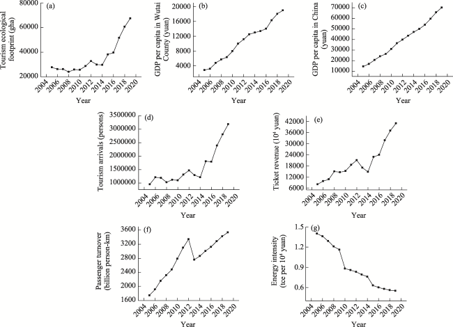
Tourism can cause serious environmental pollution due to high consumption levels. With the development of tourism in Mount Wutai, the environmental pressure has been increasing. This study explored the influences of tourist arrivals in Mount Wutai, ticket revenue from domestic tourists in Mount Wutai, national passenger turnover, energy intensity, GDP per capita in Wutai County and GDP per capita in China on the tourism ecological footprint in Mount Wutai from 2005 to 2019. The extended STIRPAT (Stochastic Impacts by Regression on Population, Affluence and Technology) model was constructed by using principal component regression. The results were as follows: (1) The tourism ecological footprint in Mount Wutai increased during the study period, from 27798.07 gha in 2005 to 67467.36 gha in 2019. (2) From 2005 to 2019, tourist arrivals in Mount Wutai, ticket revenue from domestic tourists in Mount Wutai, national passenger turnover, GDP per capita in Wutai County and GDP per capita in China grew, while energy intensity declined. (3) The extended STIRPAT model showed that the elasticity coefficients of tourist arrivals in Mount Wutai, ticket revenue from domestic tourists in Mount Wutai and national passenger turnover were 0.086%, 0.075% and 0.164%, respectively, which indicated that the tourism ecological footprint in Mount Wutai would increase by 0.086%, 0.075% and 0.164%, respectively, when those parameters increased by 1%; the elasticity coefficients of GDP per capita in Wutai County and GDP per capita in China increased at an escalating pace, but the environmental Kuznets curve did not exist, indicating that economic growth did not alleviate the environmental pressure during the study period; the elasticity coefficient of energy intensity was -0.108%, which indicated that the tourism ecological footprint would decrease by 0.108% when energy intensity increased by 1%. Therefore, the implementation of effective policies and technological innovation would significantly reduce the tourism ecological footprint in Mount Wutai.
LUO Shuzheng , YIN Jianshu , BAI Hailong , CAI Fuyan . Tracking the Drivers of the Tourism Ecological Footprint in Mount Wutai, China, based on the STIRPAT Model[J]. Journal of Resources and Ecology, 2023 , 14(5) : 1053 -1060 . DOI: 10.5814/j.issn.1674-764x.2023.05.016
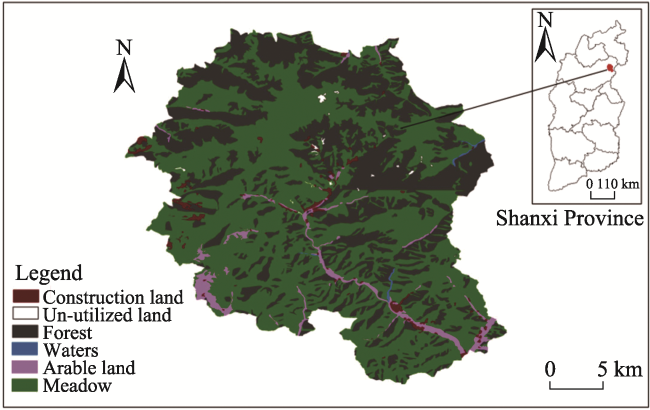
Fig. 1 The geographic location of Mount Wutai |
Table 1 The results of Spearman’s correlation analysis for the TEF and its drivers |
| Drivers of TEF | R | N | GDPc | T | PT | GDPw |
|---|---|---|---|---|---|---|
| Correlation coefficients | 0.825** | 0.914** | 0.875** | -0.875** | 0.814** | 0.875** |
| P | < 0.01 | < 0.01 | < 0.01 | < 0.01 | < 0.01 | < 0.01 |
| N | 15 | 15 | 15 | 15 | 15 | 15 |
Note: ** represents a significant correlation at the 0.01 level. |
Fig. 2 Dynamic changes in the tourism ecological footprint and its drivers in Mount Wutai |
Table 2 KMO and Bartlett’s test |
| Method | Statistic | Value |
|---|---|---|
| KMO test | Kaiser-Meyer-Olkin measure of sampling adequacy | 0.744 |
| Bartlett’s test of sphericity | Approx. Chi-Square | 414.069 |
| df | 28 | |
| P | < 0.05 |
Table 3 Total variance explained |
| Component | Initial eigenvalue | Extraction sum of squared loadings | ||||
|---|---|---|---|---|---|---|
| Total | Percentage of variance (%) | Cumulative contribution rate (%) | Total | Percentage of variance (%) | Cumulative contribution rate (%) | |
| 1 | 7.481 | 93.511 | 93.511 | 7.481 | 93.511 | 93.511 |
| 2 | 0.364 | 4.546 | 98.057 | |||
| 3 | 0.105 | 1.313 | 99.371 | |||
| 4 | 0.029 | 0.359 | 99.729 | |||
| 5 | 0.020 | 0.245 | 99.974 | |||
| 6 | 0.002 | 0.026 | 100.000 | |||
| 7 | 0.000 | 0.000 | 100.000 | |||
| 8 | 0.000 | 0.000 | 100.000 | |||
Note: The extraction method was principal component analysis. |
Table 4 Component matrix |
| Variable | Component 1 |
|---|---|
| lnGDPw | 0.986 |
| lnGDPw2 | 0.986 |
| lnN | 0.867 |
| lnT | -0.981 |
| lnR | 0.965 |
| lnGDPc | 0.994 |
| lnGDPc2 | 0.994 |
| lnPT | 0.956 |
Note: The extraction method was principal component analysis, and one component was extracted. |
Table 5 Elasticity coefficients of GDPw and GDPc |
| Year | Elasticity coefficient of GDPw | Elasticity coefficient of GDPc |
|---|---|---|
| 2005 | 0.537 | 0.782 |
| 2006 | 0.544 | 0.794 |
| 2007 | 0.568 | 0.809 |
| 2008 | 0.579 | 0.821 |
| 2009 | 0.585 | 0.827 |
| 2010 | 0.599 | 0.839 |
| 2011 | 0.613 | 0.851 |
| 2012 | 0.619 | 0.858 |
| 2013 | 0.626 | 0.864 |
| 2014 | 0.628 | 0.870 |
| 2015 | 0.630 | 0.875 |
| 2016 | 0.633 | 0.880 |
| 2017 | 0.642 | 0.888 |
| 2018 | 0.648 | 0.895 |
| 2019 | 0.651 | 0.900 |
| [1] |
|
| [2] |
|
| [3] |
|
| [4] |
|
| [5] |
|
| [6] |
|
| [7] |
|
| [8] |
|
| [9] |
|
| [10] |
|
| [11] |
|
| [12] |
|
| [13] |
|
| [14] |
|
| [15] |
|
| [16] |
|
| [17] |
|
| [18] |
|
| [19] |
|
| [20] |
|
| [21] |
|
| [22] |
|
| [23] |
|
| [24] |
|
| [25] |
|
| [26] |
|
| [27] |
|
| [28] |
|
| [29] |
|
| [30] |
|
/
| 〈 |
|
〉 |