Impact of Human Activities on Ecosystem

Can the Soil Erosion in Coastal Mountainous Areas Disturbed by Electric-transmission-line Construction be Estimated with a Deep Learning Model?

  • LI Xi , 1 ,
  • JIANG Shixiong , 1, * ,
  • ZHAO Shanshan 2 ,
  • LI Xiaomei 3 ,
  • CHEN Yao 1 ,
  • WANG Chongqing 1 ,
  • WENG Sunxian 1
Expand
  • 1. Electric Power Research Institute, State Grid Fujian Electric Power Co. Ltd, Fuzhou 350007, China
  • 2. School of Geographical Sciences/School of Carbon Neutrality Future Technology, Fujian Normal University, Fuzhou 350117, China
  • 3. College of Environmental and Resource Sciences/College of Carbon Neutral Modern Industry, Fujian Normal University, Fuzhou 350117, China
*JIANG Shixiong, E-mail:

LI Xi, E-mail:

Received date: 2023-01-30

  Accepted date: 2023-03-25

  Online published: 2023-08-02

Supported by

The State Grid Fujian Electric Power Co. Ltd.(52130420002F)

Abstract

Soil erosion monitoring in coastal mountainous areas is very important during the construction of Electric-Transmission-Line (ETL) because of the impact this disturbance has on the sensitive environment. In this study, high-resolution remote sensing data and deep learning models including Dense and Long Short-Term Memory (LSTM) were used to fit the popular soil erosion equation, which is called the Revised Universal Soil Loss Equation (RUSLE), for the Min-Yue ETL (in Fujian). The accuracy of soil erosion regression was then evaluated in the transmission line buffer area and sampling spots at two spatial scales in order to obtain the optimized parameters and a suitable model. The results show that the Dense and LSTM models can meet the accuracy requirements by using 10 characteristic values, including soil erodibility, annual rainfall, mountain vegetation index (NDMVI), DEM, slope, four bands gray values of high-spectral image, construction attributes. The optimized parameters for the priority machine-learning model LSTM are as follows: the layer depth is 3, the layer capacity is 512, the dropout ratio is 0.1, and the epoch of the LSTM model is 7060. The regression accuracy of the LSTM model decreases with an increase in soil erosion levels, and the average regression accuracy is greater than 0.98 for the slight level of soil erosion. Therefore, the machine-learning model of LSTM can be applied for quickly monitoring the soil erosion using high resolution remote sensing data.

Cite this article

LI Xi , JIANG Shixiong , ZHAO Shanshan , LI Xiaomei , CHEN Yao , WANG Chongqing , WENG Sunxian . Can the Soil Erosion in Coastal Mountainous Areas Disturbed by Electric-transmission-line Construction be Estimated with a Deep Learning Model?[J]. Journal of Resources and Ecology, 2023 , 14(5) : 1026 -1033 . DOI: 10.5814/j.issn.1674-764x.2023.05.013

1 Introduction

Soil erosion is one of the most widely distributed problems leading to land degradation. Currently, the universal soil loss equation (USLE), the revised universal soil loss equation (RUSLE) and its derived models are the most extensively used models among 435 types of soil erosion models (their representation in the literature accounts for 41%) (Ma et al., 2019; Xiong et al., 2019; Borrelli et al., 2021), and they are also commonly used in the soil loss research related
to Electric-Transmission-Line (ETLs) (Li et al., 2021; Nie et al., 2022). In the RUSLE model, R (Rainfall erosivity factor), K (Soil erodibility factor), L (Slope length factor) and S (Slope steepness factor) are relatively stable in a region, while C (Cover and management factor) and P (Support practice factor) are very sensitive to land cover, vegetation cover and soil & water conservation activities (Feng and Zhao, 2014; Zhang et al., 2015; Huang et al., 2020). Different calculation methods may lead to significant changes in the soil erosion modulus. The deep learning method shows an outstanding ability in feature learning and fitting, so it avoids the complex calculation process of soil erosion factors, and this method can return the relationships between input features and soil erosion intensity to provide the intelligent recognition of soil erosion (Jiang et al., 2021). Common deep learning models include random forest (RF), gradient hoist (GBM), integrated learning, artificial neural network, and others. (Nguyen et al., 2021; Nguyen and Chen, 2021; Wan et al., 2022). Among these methods, the convolutional neural network has shown better learning and expression abilities for image features than the other neural networks and it has gained many achievements in image classification, semantic segmentation, audio and video enhancement and other fields (Li et al., 2016). It has also been applied to calculate the regional soil erosion using images with medium spatial resolution or below (≥30 m) (Wang et al., 2022). However, the soil erosion process is closely related to spatial scale (Painting et al., 2022), and the spatial resolution of the data restricts the accuracy of soil erosion intensity estimations in construction spots. Along the southeast coast of China, the ETL network is densely built in the mountainous areas with serious terrain fluctuations and high vegetation coverage. Since the network is easily blocked by vegetation or other ground objects, the resulting images have seriously mixed pixels. Therefore, high-resolution remote sensing images are needed to accurately monitor the soil erosion on the building spots during construction. Meanwhile, because the two-dimensional window of the convolutional network may lead to interference from surrounding ground objects, it is not suitable for the intelligent training and learning of the soil erosion intensity along ETL. The need for high spatial resolution and the noise interference of deep learning algorithms have restricted the application of deep learning models in soil erosion calculations during the construction period of power transmission and transformation projects.
In this study, Skysat remote sensing images with 0.5 m spatial resolution and RUSLE were integrated into a deep learning model for soil erosion estimation in an ETL. The Dense and LSTM models were selected to regress the soil erosion modulus during the construction period of a coastal ETL. The model optimization parameters were obtained according to the cost time and the evaluation accuracy. The optimal model was determined based on the regression results at two spatial scales, one from the line buffer zone and the other from the construction area. The optimal model could directly fit the soil erosion grade according to the input soil erosion features, replace the traditional RUSLE model based on empirical parameters, and improve the computational efficiency of soil erosion and the general application of soil erosion. This model can also be used to calculate the soil erosion grade for other engineering projects with complex terrain at a small scope.

2 Study area

The Min-Yue ETL (Fig. 1) spans 72.5 km. It starts from 500 kV substation in Donglin, Zhangzhou and passes through Zhangpu, Yunxiao and Pinghe counties, in Zhangzhou, Fujian Province. It contains 150 base points, which have electric poles installed. Due to the destruction of vegetation on the surface, soil erosion is aggregated around the base points, most of which are located in the mountainous area, and they are connected as a base line from southeast to northwest. The elevation of the line ranges from 50 m to 1142 m. The area is covered by dense vegetation on the red soil and yellow-red soil. The relief is characterized by the middle-low mountain and hilly landform. The climate belongs to the subtropical marine monsoon climate, with an average annual rainfall of 1501 mm to 1796.6 mm. The ETL construction aggravates the intensity of local soil erosion in Pinghe County, which belongs to the national key control area of soil and water loss in the red soil of Fujian, Guangdong and Jiangxi.
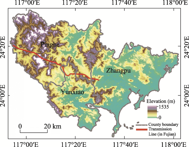
Fig. 1 Study area where the Min-Yue ETL (in Fujian) passes through

3 Data and methods

3.1 Data sources

The Skysat image used has high spatial resolution of 0.5 m and four bands of visible light and near infrared. The image date was in November 2021, and the total capacity of Skysat images of Min-Yue ETL is larger than 10 G. Images with resolution of 0.5 m were used to determine the precise construction area and to correct the land use types. Images with down-sampling resolution of 2.5 m were used for calculating the RUSLE factors. The land use type data were obtained either from the dataset on ERSI’s official website and then resampled to 2.5 m or from the Skysat image classification results. In this study, the 2.5 m Skysat image was classified to obtain land use types. DEM data were obtained from ASTER GDEM (http://www.gscloud.cn/) with 30 m resolution for the geospatial data cloud. Soil type data were from the National Data Center for Earth System Science 1:1000000 soil type map (http://www.geodata.cn/, with the spatial resolution of 1 km). DEM and Soil type images were up-sampled to 2.5 m by bilinear interpolation. Rainfall data were from the GPM rainfall dataset with spatial resolution of 0.1° (https://gpm.nasa.gov/, spatial resolution about 10 km). Monthly-Final data from January to September and Daily-Late data from Octorber 1st to December 31st in the GPM rainfall dataset for 2021 were used to summarize the annual rainfall. The correlation of the rainfall data and DEM was examined to determine whether to use Kriging interpolation or Co-Kriging interpolation and the result was then resampled to 2.5 m.

3.2 Main process

This study proposed a three-part technical process for estimating the soil erosion intensity by using deep learning models (Fig. 2). The first part was preparing the input, including 10 features connected with the ETL’s soil erosion and the soil erosion reference value from the results of RUSLE (Section 3.3). The second part was training the above data in the deep learning models (Dense model and LSTM model) for the optimized parameters (Section 3.4). Finally, the deep learning models were tested by using the untrained sampling data in both the ETL buffer zone and the construction spots (Section 3.5).
Table 1 Data and preprocessing
Data Spatial resolution Preprocessing
Skysat image 0.5 m Obtain precise construction area from an image with 0.5 m spatial resolution
and change the pixel scale to 2.5 m spatial resolution for the RULSE factors
Land use type 10 m Resample ERSI landuse type dataset to 2.5 m
2.5 m Classify the down-sampled 2.5 m image
DEM soil type image GPM 30 m Bilinear interpolation to 2.5 m
1 km Bilinear interpolation to 2.5 m
0.1° (about 10 km) 202101–202109: Monthly-Final rainfall data
20211001–20211231: Daily-Late rainfall data
$\text{Annual}\ \text{Rainfall}\And \And \text{DEM}\left\{ \begin{matrix} P~\text{value}\le 0.05:Co-Kriging\ \operatorname{int}erpolation \\ P~\text{value}0.05:\text{Kriging}\ \text{interpolation}\ \ \ \ \ \ \ \ \ \\ \end{matrix} \right.$
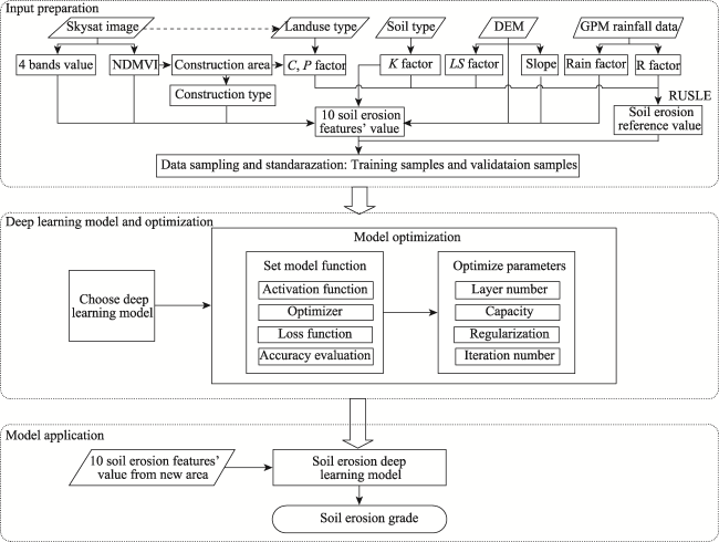
Fig. 2 Main steps in the soil erosion grade estimation by using deep learning models

3.3 Input preparation

3.3.1 Reference value of soil erosion

The Revised Universal Soil Loss Equation (RUSLE) was used to calculate the soil erosion modulus as the reference (output) value for the deep learning model.
$A=R\times K\times L\times S\times C\times P$
In formula (1), $A$ is the modulus of soil erosion (t km–2); $R$ is the rainfall erosivity factor (MJ mm ha–1 h–1 yr–1), obtained by the Kriging/Co-Kriging interpolation (Zhou et al., 1995); K is the soil erodibility factor (t ha h ha-1 MJ mm), obtained by the interpolation result of the K value in Fujian province (Fang et al., 1997) ; L is the slope length factor and $S$ is the slope steepness factor, which can be obtained by the Slope Length Factor Calculation Tool (Fu et al., 2015) ; C is the factor for vegetation cover and management, which could be obtained from the NDMVI (Normalized Difference Mountain Vegetation Index) (Wu and Xu, 2011) and the vegetation coverage was assigned by sections (Yao, 2016); and P is the support practice factor, which was obtained by the corrected land use classes in Table 2 that are suitable for the study area (Bu et al., 1997; Shi et al., 2002; Chen et al., 2014). Along the Min-Yue ETL, there are four main land use classes: forest, bare land, farmland (mostly on the mountains with slope), and other (Impermeable surface).
Table 2 Values of the P factor with slope angles for the Min-Yue ETL (in Fujian)
Land use type Bare land Forest Farmland Other
<5° 5°-10° 10°-15° 15°-20° 20°-25° >25°
Value 1 0.7 0.1 0.221 0.305 0.575 0.705 0.8 0

3.3.2 Soil erosion feature group

The soil erosion feature group (Table 3) contains the soil erosion reference value and 10 selected soil erosion parameters.
As a stable factor of the earth’s surface, K is chosen to express soil erodibility that is the same as RUSLE. The rain in coastal mountainous areas is frequent and heavy, so the annual rainfall as Rain was chosen to express the rainfall erosivity. In the Slope Length Factor Calculation Tool, DEM was used to calculated the length factor and the slope factor, so DEM was chosen to express the physical features. C is a piecewise function of NDMVI, so NDMVI was chosen to express vegetation cover and management features. P is a piecewise function of the slope and land use classes by supervised classification based on spectral bands and land use class correction by changing the land use classes in the construction area to bare land, so the four bands of grayscale for the Skysat image, the type code of construction area and the slope were used to express the soil and water conservation measure features.
Table 3 Characteristic values and sources of soil erosion features
No. Feature Remark
1 K From the K value table of Fujian
2 Rain $Rain=\left\{ \begin{matrix} 24\times \underset{i=1}{\overset{12}{\mathop \sum }}\,{{D}_{i}}{{P}_{i}},\begin{matrix} {} & {} \\ \end{matrix}\text{for}\ \text{monthly}\ \text{rainfall }\!\!~\!\!\text{ data} \\ \underset{i=1}{\overset{n}{\mathop \sum }}\,{{p}_{i}},\begin{matrix} {} & {} \\ \end{matrix}\text{for}\ \text{daily}\ \text{rainfall}\ \text{data} \\ 24\times \underset{i=1}{\overset{j}{\mathop \sum }}\,{{D}_{i}}{{P}_{i}}+\underset{i=jday+1}{\overset{n}{\mathop \sum }}\,{{p}_{i}},\text{for}\ \text{mixed}\ \text{rainfall}\ \text{data} \\ \end{matrix} \right.$
Di is the day of each month; Pi is the monthly rainfall amount per hour (mm h–1); pi is the daily rainfall amount (mm); n is the day of the year; j is the amount of monthly rainfall; and jday is the day of j months.
3 DEM ASTER GDEM
4 Slope Calculated by DEM[18]
5 NDMVI Calculated by the 3rd and the 4th bands of the Skysat image[19]
6 b1 The blue (1st) band grayscale of the Skysat image
7 b2 The green (2nd) band grayscale of the Skysat image
8 b3 The red (3rd) band grayscale of the Skysat image
9 b4 The near infrared (4th) band grayscale of the Skysat image
10 Type Set construction area as 1, and non-construction area as 2
11 A Reference value from RUSLE

3.3.3 Feature acquisition and standardization

The ratio of sample points in the non-construction area and the construction area, and the ratio of the testing sample number and validation sample number in the deep learning model are both 2:1. In this study, 8000 sample points in the construction area and 16000 sample points in the non-construction area were obtained. The soil erosion feature group values should be standardized according to formula 2 for inputting as the samples in the deep learning model:
${f}'=\left( f-mean\_f \right)/std\_f$
In formula (2), $f\text{ }\!\!~\!\!\text{ }and\text{ }\!\!~\!\!\text{ }{f}'$are the values of the soil erosion feature before and after standardization, respectively; and $mean\_f$ and $std\_f$ are the mean value and the variance of f, respectively.

3.4 Deep learning models and optimization

3.4.1 Deep learning models

The Dense model (Fully Connection, FC) is the simplest nonlinear deep learning model. Its precision can also be used as the basis for evaluating the capability of other models (e.g., LSTM). The Dense model processes nonlinear changes of input features and extracts N kinds of feature associations (N, model capacity). The formula is as follows:
$output=activation\left( Wo\times input+bo \right)$
In formula (3), input is the first 10 features in the soil erosion feature group, output is the 11th feature in the soil erosion feature group, Wo is the weight matrix, bo is the layer bias, and activation is the nonlinear function.
LSTM (Long-short term memory) is a neural network that accounts for dependencies across observations in a time series. It is a special RNN (Recurrent Neural Network), which can carry information across multiple time steps (Hochreiter et al., 1997) to solve the problem of gradient disappearance. The LSTM model adds a track carrying data to the RNN model.
$outpu{{t}_{t}}=activation\times (Wo\times inpu{{t}_{t}}+Uo\times stat{{e}_{t}}+Vo\times {{c}_{t}}+bo)$
In formula (4), t is the t-th time step; $outpu{{t}_{t}}$ and $inpu{{t}_{t}}$ are the output and input values of the t-th time step, respectively; $stat{{e}_{t}}$ and $c\_t$ are the state value and carry value of the t-th time step, respectively; $Wo,\ Uo\ \text{and}\ Vo$ are the weight matrix, the layer bias and the carry value of the t-th time step, respectively; and $activation$ is the nonlinear function.
LSTM tends to perform better than Dense for one-term data regression problems, but it does so with a higher time cost.

3.4.2 Model optimization

Model function, number of layers, capacity, regularization, number of iterations, MAE (Mean Absolute Error) and running time of the deep learning model were considered for optimizing the model parameters. After training a model using test samples, Val-MAE (MAE of validation Error) was used to determine the model accuracy.
Functions: The functions were chosen as follows: activation function as ReLU (Linear Rectification Function), optimizer as RMSProp (Root Mean Square Propagation), loss function as MSE (Mean Square Error), accuracy evaluation as MAE in the Dense model; and the choices in the LSTM model were: activation function as Tanh, optimizer as Adam (Adaptive Moment Estimation), loss function as MSE, and accuracy evaluation as MAE.
Layer number: Considering the fitting capacities and calculation amounts of the Dense and LSTM models, the layer number was set as 3.
Capacity: The capacity is determined by the capacity size and the time of a single iteration. When the capacity is larger than 512, the time of a single iteration increases dramatically in the two models, so the capacity was set to 512.
Regularization: The weight regularization enhancement effect is not good in these two models, while dropout reduces the Val-MAE significantly. When the dropout ratio is 0.1, the Val-MAE decreases the most. Therefore, the dropout regularization method was selected and the dropout ratio was set to 0.1.
Iteration number: The over-fitting point can be obtained by the minimum of Val-MAE, and the corresponding number of iterations is the moderate iteration number. As shown in Fig. 3, the number of iterations for over-fitting points in the Dense model is 185×10=1850, while the number of iterations for over-fitting points in the LSTM model is 706×10=7060.
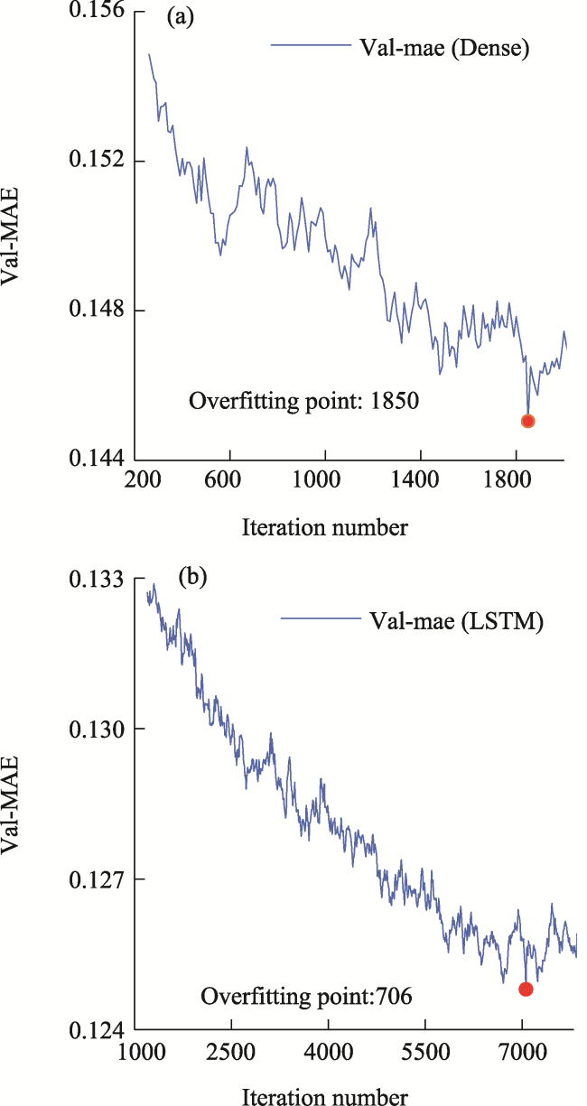
Fig. 3 Over-fitting iteration numbers of the Dense and LSTM models

3.5 Model application

In Fig. 2, based on the results of model optimization, the following settings were made: layer number as 3, capacity as 512, dropout ratio as 0.1, iteration number of the Dense and LSTM models as 1850 and 7060, respectively. These settings were used to retrain the deep learning models, in order to obtain the 11 features (in Table 2) of points within the 400-m buffer of the transmission line, and then the retrained deep learning models were used to calculate the soil erosion fitting values. The soil erosion reference values and the soil erosion fitting values were graded according to the soil erosion intensity classification grade standard SL190- 2007.

4 Research results

The accuracy of the deep learning model was evaluated at two spatial scales: a 400-m buffer of the transmission line and a 100-m buffer of the construction tower.

4.1 Accuracy in the 400-m buffer of the transmission line

There are 8162830 points with a slight erosion grade (accounting for 96.97% as the overall fitting accuracy standard), 245992 points with a mild erosion grade, 6737 points with a moderate erosion grade and 2101 point with a strong erosion grade in the 400-m buffer area. The total regression accuracies of Dense and LSTM models are 97.69% and 97.84%, respectively, so both are higher than 96.97%. The accuracies of the two models at each soil erosion grade are shown in Table 4.
Table 4 Deep learning model accuracy of the soil erosion grades in the 400-m buffer
Soil erosion grade RUSLE reference LSTM result Dense result
Area (km²) Percent (%) Area (km²) Percent (%) Error (%) Area (km²) Percent (%) Error (%)
Slight 51.02 96.97 50.80 96.56 -0.43 50.09 95.21 -1.82
Mild 1.54 2.92 1.75 3.33 13.79 2.43 4.62 58.14
Moderate 0.04 0.08 0.06 0.12 46.91 0.09 0.17 111.30
Intensity 0.01 0.02 0.00 0.00 -100.00 0.00 0.00 -100.00
The data in Table 4 show that the errors of the LSTM model are significantly lower than those of the Dense model. The errors of the two models increase with increases in the soil erosion grade. The error is less than 2% in the slight soil erosion grade but reaches -100% in the strong soil erosion intensity grade.

4.2 Accuracy in the 100-m buffer of the construction tower

Combining the overlapping buffers and deleting the non-construction buffers yielded 89 construction buffers.
The accuracy of a deep learning model in the construction buffer is defined as acc:
$ac{{c}_{ij}}={{N}_{ij}}/{{M}_{ij}}$
In formula (5), accij represents the accuracy of the j th soil erosion grade in the th buffer area, Nij represents the correct point number of the j th soil erosion grade in the i th buffer area, Mij represents the reference (RUSLE) point number of the j th soil erosion grade in the i th buffer area, and i=1, 2,…, 89; j, k=1, 2,…, 3, where 1 means slight, 2 means mild, and 3 means moderate.
The soil erosion grade accuracies of two models in the 89 construction buffers are shown in Table 5.
Table 5 Model accuracy of soil erosion grades in the construction area
Model Slight grade Mild grade Moderate grade
Min Max Average Min Max Average Min Max Average
Dense 0.83 1.00 0.98 0.07 0.96 0.72 0.01 0.86 0.43
LSTM 0.83 1.00 0.98 0.29 0.97 0.75 0.23 0.90 0.52
The accuracies of the Dense and LSTM models decrease with increases in the soil erosion grade, and the average accuracy in the slight grade is up to 0.98, while the average accuracies in the moderate grade are down to 0.43 and 0.52, respectively. Moreover, the accuracies of the soil erosion grades in the LSTM model are better than those in the Dense model in all soil erosion grades.
In total, 89 buffers show slight and mild degrees of soil erosion and 29 buffers show a moderate degree soil erosion. Dividing the accuracy into 10 levels, the accuracies of the Dense and LSTM models for slight, mild and moderate soil erosion grades in the construction buffers were counted respectively, as shown in Fig. 4.
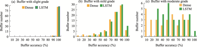
Fig. 4 Soil erosion grade accuracies of the deep learning model in the construction buffer
We defined acc above 0.8 as high precision, acc below 0.4 as low precision, and acc below 0.2 as poor precision. The results show that for the slight grade, all the buffers of the two models have high precision. For the mild grade, the LSTM model has 63 high precision buffers, accounting for 70.79%, while the Dense model only has 58 high precision buffers, accounting for 65.17%. The LSTM model has three low precision buffers, accounting for 3.37%, and the Dense model has seven low precision buffers, accounting for 7.87%, among which there are three poor precision buffers, accounting for 3.37%. For the moderate grade, the LSTM model has nine low precision buffers, accounting for 31.03%, and the Dense model has 13 low precision buffers, accounting for 44.83%, among which there are eight poor precision buffers, accounting for 27.59%.
These results indicate that the Dense model and the LSTM model have the same fitting accuracy in the two spatial scales of the 400-m transmission line buffer and the 100-m construction buffer, that is, the accuracy decreases with increases in the soil erosion grade. The accuracy is the highest, with an average accuracy of 0.98, in the slight soil erosion grade, and the average accuracy drops to about 0.50 in the moderate soil erosion grade. The LSTM model is superior to the Dense model. Buffers with accuracy below 0.2 occur in the Dense model when the soil erosion grade is above the slight grade, while the accuracies of buffers are always above 0.2 in the LSTM model. Therefore, the accuracy of the LSTM model is higher and the regression relationship is more stable than that of the Dense model.

5 Conclusions and discussion

In this study, the reference feature values calculated by the RUSLE model, the gray scale of Skysat image bands, and other related geographical parameters were used to form soil erosion feature groups in order to train the Dense model and the LSTM model. The accuracy of the deep learning model was analyzed at two spatial scales using the transmission line buffer and the construction buffer. The results provide an intelligent method of soil erosion monitoring for the transmission lines in subtropical coastal mountainous areas.
(1) The high resolution of the Skysat image was used to correct the classes in the construction area and to obtain precise C and P factors for the RUSLE model in order to calculate the soil erosion modulus as the reference value for the deep learning model. Based on 11 soil erosion features, such as reference value, four bands of grayscale in the images, K factor, DEM, slope, NDMVI, annual rainfall and construction value, the deep learning model was trained and optimized. The LSTM model was chosen to realize the intelligent monitoring of the soil erosion grade during the construction period of transmission lines, which solves the problems of too many empirical parameters and the complicated calculation process of the RUSLE model. This conclusion is consistent with the effects of deep learning algorithms in other soil erosion models (Nguyen et al., 2021; Nguyen and Chen, 2021; Wang et al., 2022).
(2) The running time cost of the LSTM model is about 2.5 times that of the Dense model, but the accuracy of the LSTM model is superior to the Dense model in all soil erosion grades. This study found that the LSTM model based on high-resolution images is more suitable for the dynamic estimation of soil erosion generated by construction projects in subtropical coastal mountainous areas. The optimal parameters of the LSTM model for transmission line soil erosion in the study area are as follows: layer number=3, capacity=512, dropout ratio=0.1, and iteration number=7060.
(3) The accuracy of the deep learning model is closely related to the samples. In the study area, the main soil erosion grade is the slight grade (96.97%), while the proportion of the soil erosion grade above the moderate level is rather small (below 0.1%). As a result, the fitting accuracy of the LSTM model is higher in the slight grade, while the deviation becomes larger in the moderate grade. There are three feasible directions for improving the applicability of the deep learning model by adjusting the samples of soil erosion grades in further studies. Firstly, the construction period should be considered. The acquired Skysat images for November 2021 are in the early part of the erosion season, while the later season from March to April in 2022 is the most prominent and serious soil erosion stage, in which more samples above the moderate soil erosion grades could be used for deep learning model training. Secondly, the sampling boundary could be limited within a certain buffer around construction area to increase the percentage of samples above the moderate soil erosion grade. Lastly, random sampling with the average number of samples for each soil erosion grade would be more moderate than that for all the soil erosion grades.
[1]
Borrelli P, Alewell C, Alvarez P, et al. 2021. Soil erosion modelling: A global review and statistical analysis. Science of the Total Environment, 780: 146494. DOI: 10.31223/X5GS3T.

[2]
Bu Z H, Sun J Z, Zhou F J, et al. 1997. Study on quantitative remote sensing method of soil and water loss and its application. Acta Pedologica Sinica, 34(3): 235-245. (in Chinese)

[3]
Chen S X, Yang X C, Xiao L L, et al. 2014. Study on soil erosion in southern hilly and mountainous areas based on RUSLE Model. Resource Science, 36(6): 1288-1297. (in Chinese)

[4]
Fang G Q, Ruan F S, Wu X H, et al. 1997. Preliminary study on erodibility characteristics of main soils in Fujian Province. Fujian Soil and Water Conservation, (2): 19-23. (in Chinese)

[5]
Feng Q, Zhao W W. 2014. Research progress of vegetation cover and management factors in USLE/RUSLE. Acta Ecologica Sinica, 34(16): 4461-4472. (in Chinese)

[6]
Fu S H, Liu B Y, Zhou G Y, et al. 2015. Slope length slope factor calculation tool. Science of Soil and Water Conservation, 13(5): 105-110. (in Chinese)

[7]
Hochreiter S, Schmidhuber J. 1997. Long short-term memory. Neural Computation, 9(8): 1735-1780.

[8]
Huang J, Yao Z H, Zha S X, et al. 2020. Research progress on soil and water conservation measures in USLE/RUSLE. Soil and Water Conservation in China, (3): 37-39, 56. (in Chinese)

[9]
Jiang D W, Jiang X W, Zhou Z L. 2021. Artificial intelligence for soil and water conservation information supervision technology support. Journal of Soil and Water Conservation, 35(4): 1-6. (in Chinese)

[10]
Li L, Hou X X, Chen X F, et al. 2021. Research on key technology of soil erosion control of transmission line project in hilly area. IOP Conference Series: Earth and Environmental Science, 831: 1-4.

[11]
Li Y D, Hao Z B, Lei H. 2016. A review of convolution neural networks. Journal of Computer Applications, 36(9): 2508-2515, 2565. (in Chinese)

[12]
Ma L, Bu Z H, Liang W G, et al. 2019. Study on quantitative monitoring method and application of soil and water loss based on USLE principle and 3S Technology. Acta Pedologica Sinica, 56(3): 602-614.

[13]
Ministry of Water Resources of the People’s Republic of China. 2008. Soil erosion classification standard SL190-2007 (SL190-2007 instead of SL190-96). Beijing, China: China Water Conservancy and Hydropower Press. (in Chinese)

[14]
Nguyen K A, Chen W, Lin B S, et al. 2021. Comparison of ensemble machine learning methods for soil erosion pin measurements. International Journal of Geo-information, 10: 42. DOI: 10.3390/ijgi10010042.

[15]
Nguyen K A, Chen W. 2021. DEM- and GIS-based analysis of soil erosion depth using machine learning. International Journal of Geo-information, 10: 452. DOI: 10.3390/ijgi10070452.

[16]
Nie H Y, Feng H, Wang W L, et al. 2022. Erosion environment and soil erosion characteristics of power transmission and transformation in hilly areas. Research of Soil and Water Conservation, 29(2): 50-56. (in Chinese)

[17]
Painting K, Zhang K L. 2022. Research Progress on scale effect of soil and water loss in China based on metrology. Ecology and Environment Sciences, 31(7): 1489-1498.

[18]
Shi Z H, Cai C F, Ding S W, et al. 2002. Study on soil and water conservation planning of farmland in small watershed based on GIS and RUSLE. Transactions of the Chinese Society of Agricultural Engineering, 18(4): 172-175. (in Chinese)

[19]
Wan L, Li S, Chen Y, et al. 2022. Application of deep learning in land use classification for soil erosion using remote sensing. Frontiers in Earth Science, 10: 849531. DOI: 10.3389/feart.2022.849531.

[20]
Wang S T, Shi M C, Chen C Y, et al. 2022. Spatial distribution of soil erosion in Hubei Province based on deep learning. Science of Soil and Water Conservation, 6(3): 119-125. (in Chinese)

[21]
Wu Z J, Xu H Q. 2011. Construction and application analysis of mountain vegetation index based on satellite image data. Journal of Geo-Information Science, 13(5): 656-664. (in Chinese)

[22]
Xiong M, Sun R, Chen L. 2019. Global analysis of support practices in USLE-based soil erosion modeling. Progress in Physical Geography, 43(3): 391-409.

[23]
Yao X. 2016. Study on remote sensing reconstruction of vegetation cover and management factor (C factor) in soil and water loss area of southern red soil. Diss., Fuzhou, China: Fujian Agriculture and Forestry University. (in Chinese)

[24]
Zhang C, Xu H Q, Zhang H, et al. 2015. Fractional vegetation cover change and its ecological effect assessment in a typical reddish soil region of southeastern China: Changting County, Fujian Province. Journal of Natural Resources, 30(6): 917-927. (in Chinese)

[25]
Zhou F J, Chen M H, Lin F X, et al. 1995. Rainfall erosivity index R value in Fujian Province. Journal of Soil and Water Conservation, 1(9): 13-18.

Outlines

/