
Journal of Resources and Ecology >
Remote Sensing Estimation Methods for Determining FVC in Northwest Desert Arid Low Disturbance Areas based on GF-2 Imagery
|
XUE Xinyue, E-mail: 1033824490@qq.com |
Received date: 2022-08-20
Accepted date: 2023-03-02
Online published: 2023-07-14
Supported by
Key Research and Development Program of China(2017YFC0504406)
Fractional vegetation cover (FVC) is a vital indicator of surface vegetation. Studies of regional vegetation cover are helpful for understanding the status of the regional ecological environment and can provide important references for the formulation of ecological restoration plans and the evaluation of restoration effects. In vegetation cover related research, studies on extraction methods have attracted much attention. Studies have shown that the universality of vegetation cover extraction methods is poor, as well as the existing studies were mostly conducted on agricultural and forest land in wet, semi-humid and semi-arid areas, while few have investigated arid areas with sparse vegetation that is mainly shrubs and grass. To investigate the accuracy and applicability of different methods for estimating vegetation cover in the near-natural zone of the northwest arid desert, this study extracted six vegetation indices (NDVI, SAVI, MSAVI, ARVI, EVI, and MVI), which could effectively exclude soil and meteorological information to obtain pure vegetation information based on GF-2 multispectral-panchromatic fusion images. Two types of models were then established, including the single VI models (DP model) and multi-VI models (R model, RF model and PCA model), three statistics (SSE, R2, RMSE) were introduced to validate model accuracy and four-fold cross-validation was used to probe the models for overfitting. After filtering the models through these methods, the selected model was applied to invert the vegetation coverage in the study area. The results show three key aspects of this system. (1) Among the various models, the DP model constructed using the EVI and the RF model are more suitable for FVC extraction in the study area. This conclusion was further verified by the significant correlation between the inversion results of the FVC for the entire study area by applying these two models. (2) The values of pure bare soil and vegetation pixels (VIs and VIv) in the DP model will obviously affect the accuracy of the model. Thus, the empirical values should not be blindly adopted in actual research. (3) The vegetation distributions in the figures of the FVC results are similar to the outline of the mountains in the study area, indicating that the coverage distribution may be greatly affected by topographic factors. It is recommended that this aspect should be introduced in subsequent studies.
Key words: FVC; GF-2; random forest model
XUE Xinyue , GUO Xiaoping , XUE Dongming , MA Yuan , YANG Fan . Remote Sensing Estimation Methods for Determining FVC in Northwest Desert Arid Low Disturbance Areas based on GF-2 Imagery[J]. Journal of Resources and Ecology, 2023 , 14(4) : 833 -846 . DOI: 10.5814/j.issn.1674-764x.2023.04.016
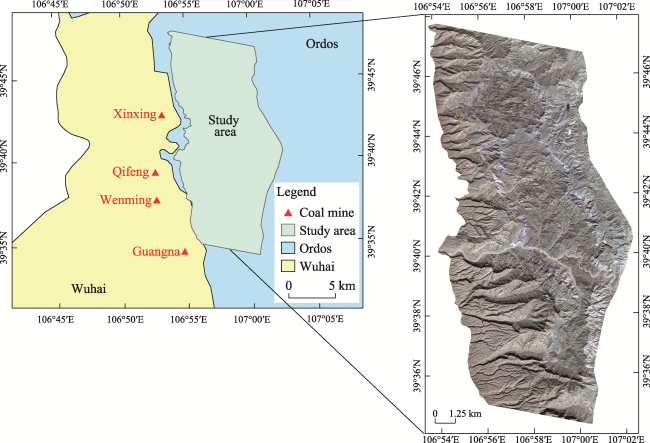
Fig. 1 Study area |
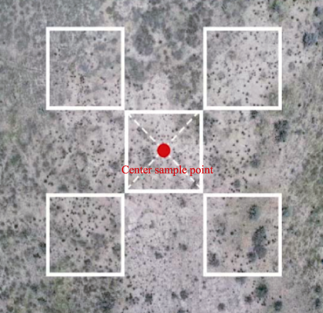
Fig. 2 Five-point sampling method |
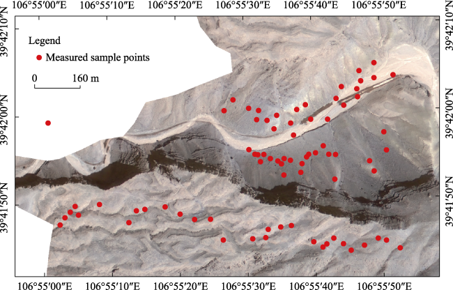
Fig. 3 Distribution of sample points for the actual measurements |
Table 1 Image Information |
| No. | Satellite | Sensor | Product level | Acquisition date | Longitude of scenic center (E) | Latitude of scenic center (N) |
|---|---|---|---|---|---|---|
| 1 | GF2 | PMS2 | LEVEL1A | 2021-08-07 | 107° | 39.84° |
| 2 | GF2 | PMS2 | LEVEL1A | 2021-08-07 | 106.94° | 39.67° |
| 3 | GF2 | PMS2 | LEVEL1A | 2021-08-07 | 106.88° | 39.49° |
Table 2 Calculation formulas of the vegetation indexes (VIs) |
| Vegetation index | Calculation method | Formula serial number | Index range | Citation | Features |
|---|---|---|---|---|---|
| NDVI | NDVI=$\frac{NIR-R}{NIR+R}$ | (2) | [-1, 1] | Rouse et al., 1973 | Ability to eliminate most variations in irradiance related to instrument calibration, sun angle, topography, cloud shadows and atmospheric conditions (most widely used) |
| SAVI | SAVI=$\frac{NIR-R}{NIR+R+L}\left( 1+L \right)$ | (3) | [-1, 1] | Huete, 1988 | The soil brightness index L was introduced to create a simple model that could properly describe the soil-vegetation system. Huete (1988) suggested that L be taken as 0.5 |
| MSAVI | MSAVI=$\frac{2NIR+1-\sqrt{{{\left( 2NIR+1 \right)}^{2}}-8\left( NIR-R \right)}}{2}$ | (4) | [-1, 1] | Qi et al., 1994 | Reduces the effect of bare soil in SAVI, and its L value can be automatically adjusted with the vegetation density, better at eliminating the soil background effect |
| ARVI | ARVI=$\frac{NIR-2R+B}{NIR+2R-B}$ | (5) | [-1, 1] | Kaufman and Tanre, 1992 | Reduces sensitivity to atmospheric effects by normalizing radiation in the blue, red and near-infrared bands and corrects remote sensing data for molecular scattering and ozone absorption |
| EVI | EVI=$\frac{2.5\left( NIR-R \right)}{NIR+6R-7.5B+1}$ | (6) | [-1, 1] | Bannari et al., 1995 | Enhances the vegetation signal by adding a blue band to correct the effect of soil background and aerosol scattering, more suitable for dense vegetation areas |
| MVI | MVI=$\sqrt{\frac{NIR-R}{NIR+R+0.5}}$ | (7) | [0, 1] | McDaniel and Haas, 1982 | Eliminates or weakens the effect of soil background on vegetation reflectance |
Note: NIR, R and B are the reflectances of the features in the near-infrared, red and blue bands, respectively. L is the soil brightness index between 0 and 1, usually taken as 0.5. |
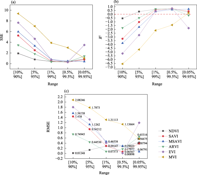
Table 3 DN value statistics based on the value intervals of [NDVIs, NDVIv] |
| DN value | [10%, 90%] | [5%, 95%] | [1%, 99%] | [0.5%, 99.5%] | [0.05%, 99.95%] |
|---|---|---|---|---|---|
| NDVI | [0.051322, 0.133003] | [0.040184, 0.155279] | [0.02162, 0.203545] | [0.010482, 0.225821] | [‒0.030358, 0.34463] |
| SAVI | [‒0.004837, 0.182795] | [‒0.005689, 0.216203] | [‒0.006371, 0.283018] | [‒0.006456, 0.316426] | [‒0.034355, 0.477896] |
| MSAVI | [‒0.005421, 0.215431] | [‒0.006424, 0.2482] | [‒0.007227, 0.320291] | [‒0.007227, 0.346506] | [‒0.046718, 0.484134] |
| ARVI | [‒0.092250, ‒0.009038] | [‒0.098194, 0.008793] | [‒0.116025, 0.056343] | [‒0.121969, 0.092006] | [‒0.1398, 0.228712] |
| MVI | [0.000958, 0.350775] | [0.000479, 0.378963] | [0.0000958, 0.435337] | [0.00004791, 0.460393] | [0.000004791, 0.566878] |
| EVI | [‒0.009418, 0.309804] | [‒0.01062, 0.364706] | [‒0.01158, 0.513725] | [‒0.0117, 0.631373] | [‒1, 0.992157] |
Table 4 VIF values between VIs |
| VIF values | Remaining variables | |||||
|---|---|---|---|---|---|---|
| SAVI | MSAVI | ARVI | EVI | MVI | ||
| NDVI | 14859.03 | 24919.92 | 251.70 | 408.94 | 1566.37 | |
| SAVI | 276.82 | 250.61 | 408.75 | 159.06 | ||
| MSAVI | 248.70 | 383.12 | 39.92 | |||
| ARVI | 16.30 | 16.30 | ||||
| EVI | - |
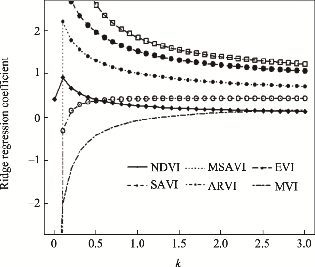
Fig. 4 Ridge trace curves |
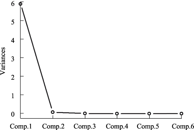
Fig. 5 Gravel map of the PCA model |
Table 5 Cumulative variance contributions of the principal components |
| Principal components | Feature root | Contribution rate (%) | Cumulative contribution rate (%) |
|---|---|---|---|
| 1 | 2.4303820 | 98.4459 | 98.4459 |
| 2 | 0.2863041 | 1.3662 | 99.8121 |
| 3 | 0.0987407 | 0.1625 | 99.9746 |
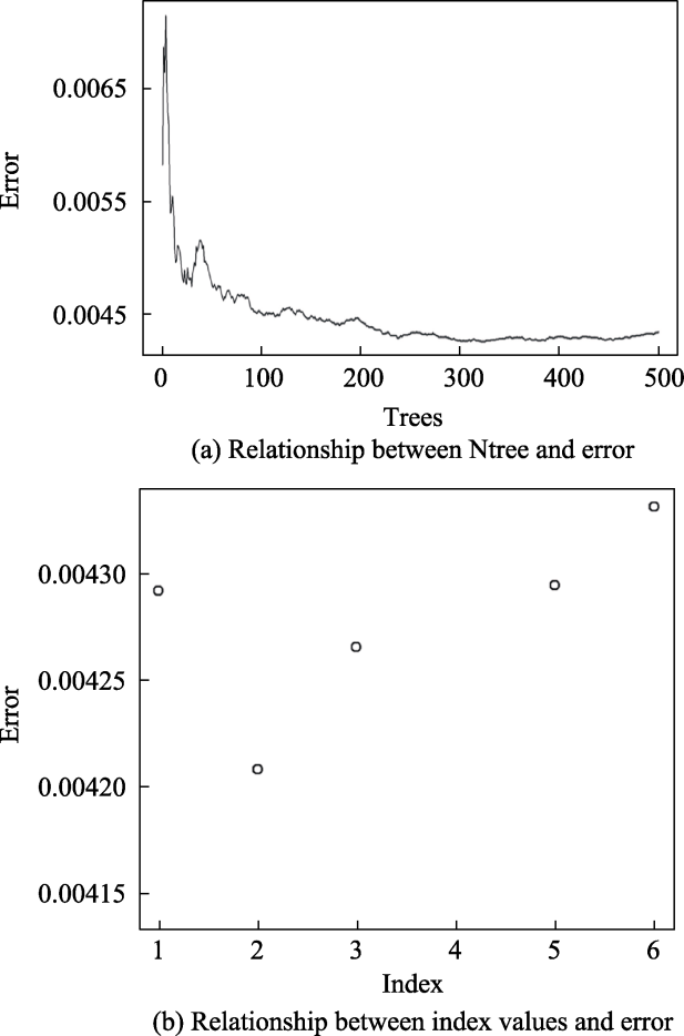
Fig. 6 Significant variables of the decision tree model |
Fig. 7 Evaluation of the accuracy of the DP model |
Table 6 The statistics of five VIs (excluding MVI) under their optimal intervals |
| VIs with optimal interval | NDVI $\left[ 0.5\text{ }\!\!%\!\!\text{ },\ 99.5\text{ }\!\!%\!\!\text{ } \right]$ | SAVI $\left[ 0.5\text{ }\!\!%\!\!\text{ },\ 99.5\text{ }\!\!%\!\!\text{ } \right]$ | MSAVI $\left[ 0.05\text{ }\!\!%\!\!\text{ },\ 99.95\text{ }\!\!%\!\!\text{ } \right]$ | ARVI $\left[ 1\text{ }\!\!%\!\!\text{ },\ 99\text{ }\!\!%\!\!\text{ } \right]$ | EVI $\left[ 0.5\text{ }\!\!%\!\!\text{ },\ 99.5\text{ }\!\!%\!\!\text{ } \right]$ |
|---|---|---|---|---|---|
| SSE | 0.4053296 | 0.2824413 | 0.3928578 | 0.3657897 | 0.2897076 |
| R2 | 0.672436 | 0.7717473 | 0.682515 | 0.7043899 | 0.765875 |
| RMSE | 0.2781874 | 0.0656734 | 0.067913 | 0.0737328 | 0.0089758 |
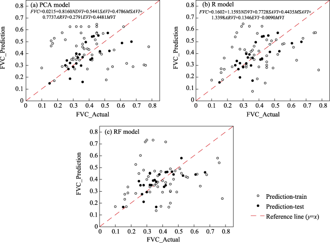
Fig. 8 Model prediction scatter plots for the PCA, R and RF models |
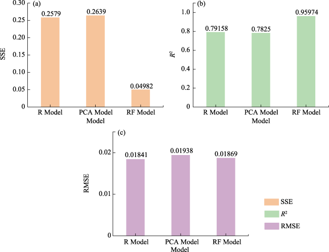
Fig. 9 Model accuracy evaluation of the PCA, R and RF models |
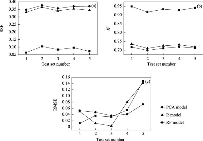
Fig. 10 Five-fold cross-validation results |
Table 7 Means of the cross-validation results |
| Model | $\overline{\text{SSE}}$ | ${{\bar{R}}^{2}}$ | $\overline{\text{RMSE}}$ |
|---|---|---|---|
| PCA | 0.364548 | 0.712160 | 0.050014 |
| R | 0.347112 | 0.724601 | 0.057356 |
| RF | 0.084036 | 0.933460 | 0.056530 |
Table 8 Statistics of the single VI & muti-VI models |
| Model type | VI | SSE | R2 | RMSE |
|---|---|---|---|---|
| DP model | $\text{SAV}{{\text{I}}_{\left[ 0.5\text{ }\!\!%\!\!\text{ },\ 99.5\text{ }\!\!%\!\!\text{ } \right]}}$ | 0.282441 | 0.771747 | 0.065673 |
| DP model | $\text{EV}{{\text{I}}_{\left[ 0.5\text{ }\!\!%\!\!\text{ },\ 99.5\text{ }\!\!%\!\!\text{ } \right]}}$ | 0.289708 | 0.765875 | 0.008976 |
| RF model | Six VIs | 0.049816 | 0.959742 | 0.018689 |
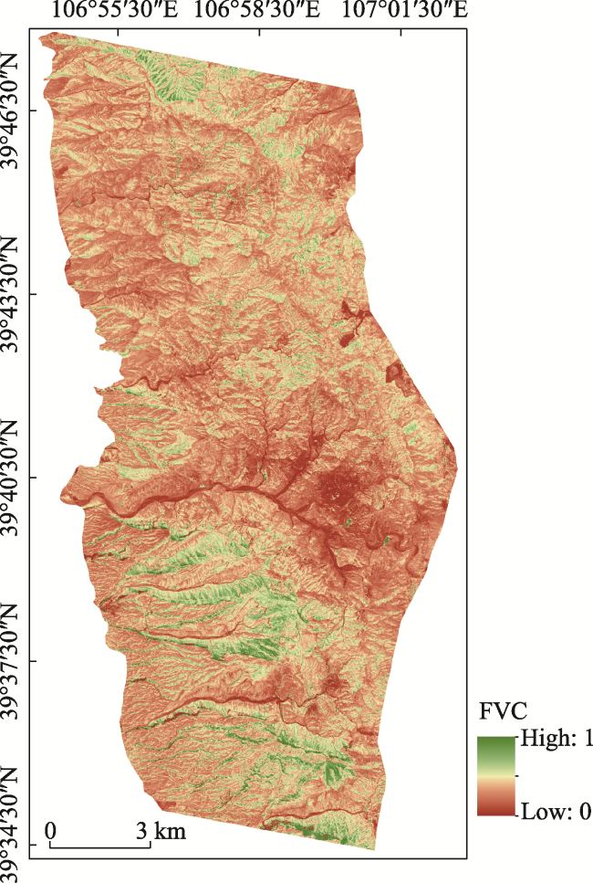
Fig. 11 The FVC result of the study area (DP model based on EVI) |
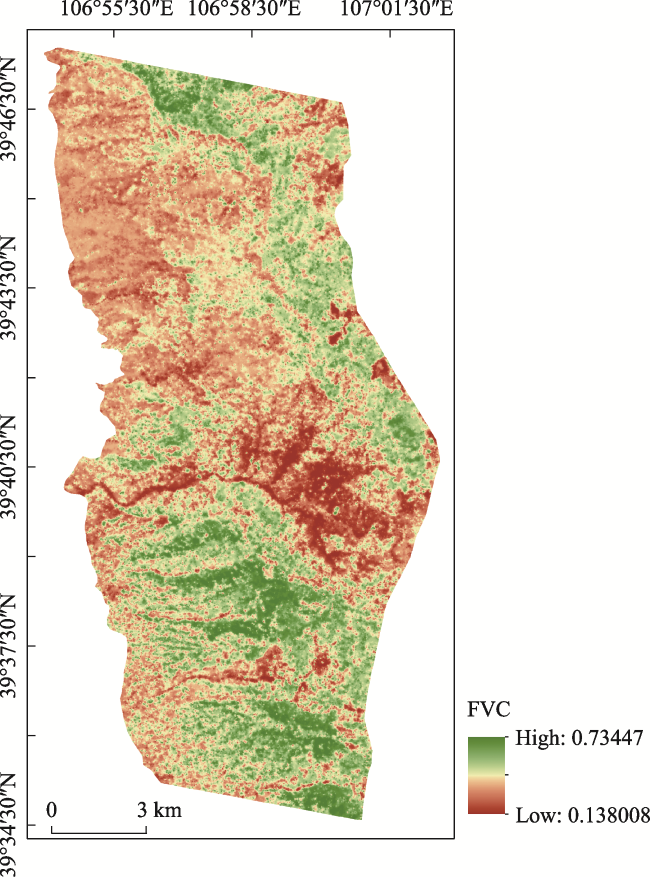
Fig. 12 The FVC result of the study area (RF model) |
| [1] |
|
| [2] |
|
| [3] |
|
| [4] |
|
| [5] |
|
| [6] |
|
| [7] |
|
| [8] |
|
| [9] |
|
| [10] |
|
| [11] |
|
| [12] |
|
| [13] |
|
| [14] |
|
| [15] |
|
| [16] |
|
| [17] |
|
| [18] |
|
| [19] |
|
| [20] |
|
| [21] |
|
| [22] |
|
| [23] |
|
| [24] |
|
| [25] |
|
| [26] |
|
| [27] |
|
| [28] |
|
| [29] |
|
| [30] |
|
| [31] |
|
| [32] |
|
| [33] |
|
| [34] |
|
| [35] |
|
| [36] |
|
| [37] |
|
| [38] |
|
| [39] |
|
| [40] |
|
| [41] |
|
| [42] |
|
| [43] |
|
| [44] |
|
| [45] |
|
| [46] |
|
| [47] |
|
| [48] |
|
| [49] |
|
| [50] |
|
| [51] |
|
| [52] |
|
| [53] |
|
| [54] |
|
| [55] |
|
| [56] |
|
| [57] |
|
| [58] |
|
| [59] |
|
| [60] |
|
/
| 〈 |
|
〉 |