
Journal of Resources and Ecology >
Vegetation Coverage Inversion based on Combined Active and Passive Remote Sensing: A Case Study of the Baiyangdian-Daqinghe Basin
|
YANG Jin, E-mail: yj3190604@bjfu.edu.cn |
Received date: 2022-05-23
Accepted date: 2022-08-20
Online published: 2023-04-21
Supported by
The National Science and Technology Major Project of the Ministry of Science and Technology of China(2018ZX07110001)
Due to poor penetrability, optical remote sensing can not identify understory vegetation beneath the canopy. Thus, the vegetation coverage extracted by optical remote sensing alone could not sufficiently capture understory vegetation information to formulate the vegetation coverage factor for soil erosion evaluation. To address this issue, the authors took the Baiyangdian-Daqing River Basin as the research object and considered the photon counting ICESat-2/ATLAS vegetation coverage sampling under different photon point classifications. Based on the measured data, satellite-ground collaborative vegetation coverage sampling was achieved in the study area. The results showed that compared with the inversion results extracted by the traditional NDVI pixel dichotomy, the vegetation coverage estimated by the random forest regression model constructed in this study was more accurate. To a certain extent, the proposed model can monitor the understory vegetation of dense forests and complement the lack of understory vegetation signal in optical remote sensing. In the three error tolerance 0.05, 0.1, and 0.15 ranges, the inversion accuracy of vegetation coverage was increased by -4.1%, 5.3%, and 9.4%, reaching the accuracy of 55.6%, 71.1%, and 94.3%, respectively.
YANG Jin , SHI Mingchang , YANG Jianying , CHENG Fu , YU Hongfeng . Vegetation Coverage Inversion based on Combined Active and Passive Remote Sensing: A Case Study of the Baiyangdian-Daqinghe Basin[J]. Journal of Resources and Ecology, 2023 , 14(3) : 591 -603 . DOI: 10.5814/j.issn.1674-764x.2023.03.014
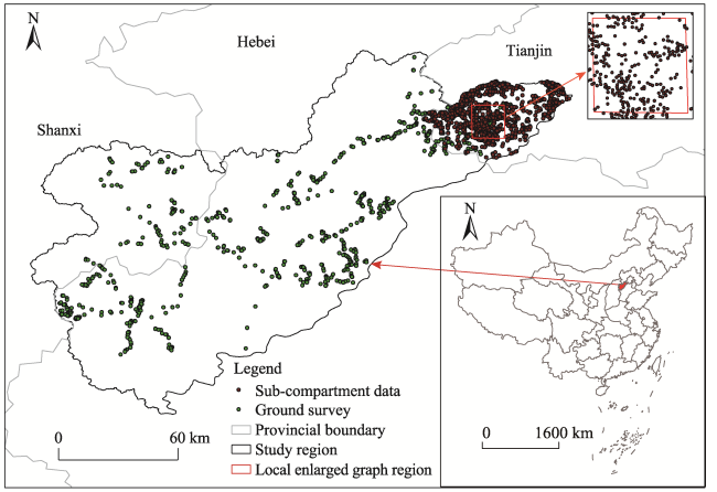
Fig. 1 Scope of the study area and distribution of the quadrat |
Table 1 Data details |
| Data types | Description | Data source | Function |
|---|---|---|---|
| Field survey data | Ground survey/Sub-compartment data | field survey | Sampling and Verification |
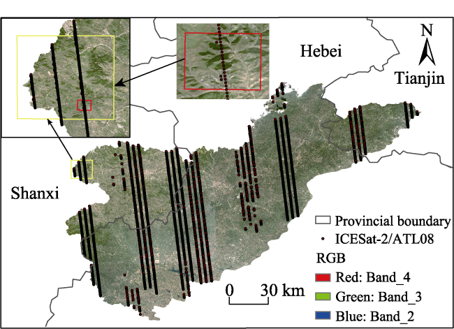
| Spaceborne lidar | ICESat-2-ATL03/ATL08 | https://nsidc.org/data/icesat-2 | Vegetation coverage sampling |
| Optical remote sensing | Sentinel-2 | Google earth engine (GEE) | Extracting feature variables for vegetation coverage inversion modeling |
| Synthetic aperture radar (SAR) | Sentinel-1 | Google earth engine (GEE) | |
| Terrain data | ALOS DEM | https://search.asf.alaska.edu/ | |
| Land use data | CGLS-LC100 | Google earth engine (GEE) | Analysis of vegetation coverage sampling results and Modeling of vegetation coverage |
Table 2 List of ICESat-2/ATL03 and ICESat-2/ATL08 data |
| Order number | ICESat-2 data product name used in research |
|---|---|
| 1 | ATL03/8_20190623194316_13220302_004_01.h5 |
| 2 | ATL03/8_20190722181912_03770402_004_01.h5 |
| 3 | ATL03/8_20190726181055_04380402_004_01.h5 |
| 4 | ATL03/8_20190816170341_07580402_004_01.h5 |
| 5 | ATL03/8_20190820165523_08190402_004_01.h5 |
| 6 | ATL03/8_20190824164704_08800402_004_01.h5 |
| 7 | ATL03/8_20190914153947_12000402_004_01.h5 |
| 8 | ATL03/8_20190918153128_12610402_004_01.h5 |
| 9 | ATL03/8_20190922152309_13220402_004_01.h5 |
| 10 | ATL03/8_20190926151450_13830402_004_01.h5 |
Fig. 2 Distribution of ICESat-2/ATLAS laser points |
Table 3 The calculation of vegetation indexes |
| Vegetation index | Calculation formula | Quantity |
|---|---|---|
| Normalized difference vegetation index | NDI(i,j)=(Bi-Bj)/(Bi+Bj), where i, j=2,$\cdots$, 8, 8A, 11, 12; i≠j and i>j | 45 |
| Ratio vegetation index | SR(i,j)= Bi/Bj, where i, j=2, $\cdots$, 8, 8A, 11, 12; i≠j | 90 |
| Enhanced vegetation index | EVI=2.5×(B8-B4)/(B8+6B4-7.5B2+1) | 1 |
| Transformed normalized vegetation index | TNDVI$=\sqrt{\left( \text{B}8-\text{B}4 \right)/\left( \text{B}8+\text{B}4 \right)+0.5}$ | 1 |
| Renormalized vegetation index | RDVI$=\left( \text{B}8-\text{B}4 \right)/\sqrt{\text{B}8+\text{B}4}$ | 1 |
| Global environmental detection index | GEMI=a×(1-0.25×a)-(B4-0.125)/(1-B4), where a=[2×(B8A2-B42)+1.5×B8A+ 0.5×B4]/(B8A+B4+0.5) | 1 |
| Soil adjusted vegetation index | SAVI=1.5×(B8-B4)/(B8+B4+0.5) | 1 |
| Adjustable vegetation index for transformed soil | TSAVI=0.5×(B8-0.5×B4-0.5)/(0.5×B8+B4-0.15) | 1 |
| Red edge chlorophyll index | CI=B7/B5-1 | 1 |
| Red edge position index | REP=705+35×[(B4+B7)/2-B5]/(B6-B5) | 1 |
| Plant senescence reflectance index | PSRI=(B4-B3)/B6 | 1 |
| Normalized vegetation canopy shadow index | NDCSI(i)=NDVI×(Bi-Bimin)/(Bimax-Bimin), where NDVI=(B8-B4)/(B8+B4), where i=5, 6, 7 | 3 |
| Normalized radar vegetation index | NDVHVV=(VH-VV)/(VH+VV) | 1 |
| Ratio radar vegetation index | RAVHVV=VV/VH | 1 |
Note: Bi: The band i in Sentinel-2; Bimin: The minimum value at Bi band in Sentinel-2; Bimax: The maximum value at Bi band in Sentinel-2; VH: The backscattering intensity in Sentinel-1 under VH polarization; VV: The backscattering intensity in Sentinel-1 under VV polarization. |
Table 4 Terrain factor feature variables |
| Terrain factor | Description |
|---|---|
| H | Elevation |
| S | Slope |
| SinA | Sine in aspect, Eastward degree |
| CosA | Cosine in aspect, Northward degree |
Note: A: Aspect. |
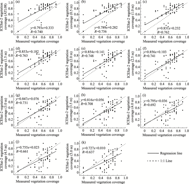
Fig. 3 Scatter plot of ICESat-2 vegetation coverage based on photon point classification and measured vegetation coverageNote: FVC_ICESat (ATL08) is the ICESat-2 vegetation cover under ATL08 photon point classification; FVC_ICESat (i) is the vegetation coverage of ICESat-2 under i high threshold photon point classification; R is the correlation coefficient between ICESat-2 vegetation coverage and measured vegetation coverage. |
Table 5 Accuracy of vegetation coverage estimation models based on the random forest regression model and NDVI pixel dichotomy |
| Methods | RMSE | EA (e<0.05) | EA (e<0.1) | EA (e<0.15) |
|---|---|---|---|---|
| RF | 0.086 | 55.6% | 71.1% | 94.3% |
| NDVI | 0.102 | 59.7% | 65.8% | 84.9% |
| AI | 0.026 | -4.1% | 5.3% | 9.4% |
Note: RF: random forest regression model, NDVI: NDVI pixel dichotomy model, AI: accuracy improvement. |
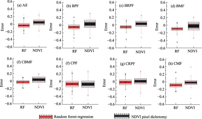
Fig. 4 Estimation of vegetation coverage error box diagram based on random forest regression and NDVI pixel dichotomyNote: (a) All: ground survey; (b) BPF: Broad-leaved pure forest; (c) BRPF: Broad-leaved relative pure forest; (d) BMF: Broad-leaved mixed forest; (e) CBMF: Coniferous and broad-leaved mixed forest; (f) CPF: Coniferous pure forest; (g) CRPF: Relatively pure coniferous forest; (h) CMF: Coniferous mixed forest. |
Fig. 5 ICESat-2 point cloud distribution map for different land-use types |
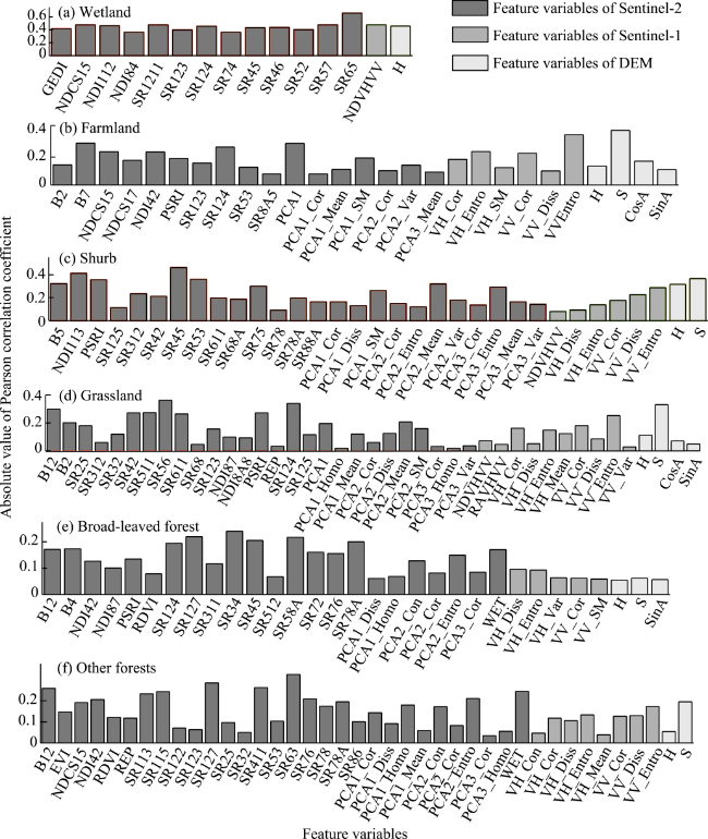
Fig. 6 Optimization results of features variables under different vegetation typesNote: PCAi_j is the texture features j of principal component i of Sentinel-2, where i=1, 2, 3; Cor: Correlation; Con: Contrast; Var: Variance; Entro: Entroy; Homo: Homogeneity; Diss: Dissimilarity; SM: Second moment. |
Table 6 Accuracy evaluation of the random forest regression model and the NDVI pixel dichotomy model in different forests |
| TSS | Methods | RMSE | EA (e<0.05) (%) | EA (e<0.1)(%) | EA (e<0.15)(%) |
|---|---|---|---|---|---|
| RF | 0.114 | 58.50 | 64.20 | 82.90 | |
| BPF | NDVI | 0.152 | 39.80 | 52.80 | 70.70 |
| AI | 0.038 | 18.70 | 11.40 | 12.20 | |
| RF | 0.108 | 63.70 | 75.60 | 88.90 | |
| BRPF | NDVI | 0.126 | 49.60 | 63.70 | 80.70 |
| AI | 0.018 | 14.10 | 11.90 | 8.20 | |
| RF | 0.109 | 51.30 | 61.80 | 88.20 | |
| BMF | NDVI | 0.141 | 46.10 | 48.70 | 63.20 |
| AI | 0.032 | 5.20 | 13.10 | 25.00 | |
| RF | 0.075 | 78.60 | 85.70 | 89.30 | |
| CBMF | NDVI | 0.100 | 60.70 | 64.30 | 85.70 |
| AI | 0.025 | 17.90 | 21.40 | 3.50 | |
| RF | 0.123 | 40.70 | 49.70 | 75.00 | |
| CPF | NDVI | 0.147 | 43.10 | 49.20 | 66.00 |
| AI | 0.024 | -2.40 | 0.50 | 9.00 | |
| RF | 0.129 | 55.80 | 64.10 | 76.90 | |
| RPCF | NDVI | 0.134 | 48.10 | 60.30 | 77.60 |
| AI | 0.005 | 7.70 | 3.80 | -0.70 | |
| RF | 0.132 | 41.90 | 48.40 | 74.20 | |
| CMF | NDVI | 0.138 | 64.50 | 77.40 | 80.60 |
| AI | 0.006 | -22.60 | -31.00 | -6.40 |
Note: TSS: Tree species structure; BPF: Broad-leaved pure forest; BRPF: Broad-leaved relative pure forest; BMF: Broad-leaved mixed forest; CBMF: Coniferous and broad-leaved mixed forest; CPF: Coniferous pure forest; RPCF: Relatively pure coniferous forest; CMF: Coniferous mixed forest; RF: Random forest regression model; NDVI: NDVI pixel dichotomy model; AI: Accuracy improvement. |
Table 7 Parameters in random forest modeling |
| Vegetation type | Sampling numbers | Num | Max_features |
|---|---|---|---|
| Farmland | 772 | 27 | 6 |
| Shurb | 1087 | 33 | 6 |
| Grassland | 7724 | 41 | 7 |
| Wetland | 33 | 15 | 4 |
| DBF | 1308 | 31 | 6 |
| OF | 4971 | 40 | 7 |
Note: DBF: Deciduous broad-leaved forest; OF: Other forests; Num: The number of feature variables; Max_features: The max features in random forest modeling. |
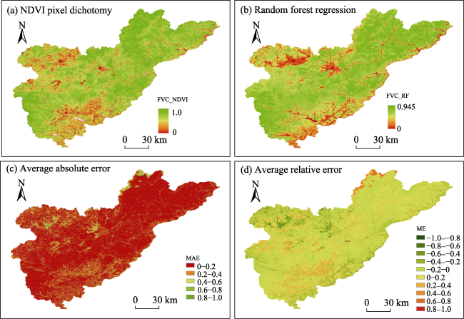
Fig. 7 Vegetation coverage inversion results and differences between random forest and NDVI pixel dichotomy model |
Table 8 Comparison of extraction results of the random forest regression model and the NDVI pixel dichotomy model in different vegetation types |
| Land cover types | Shrub | Herb | Farmland | EC | DB | OF |
|---|---|---|---|---|---|---|
| FVCME | 0.021 | 0.041 | -0.163 | -0.089 | -0.069 | -0.063 |
| FVCMAE | 0.145 | 0.141 | 0.256 | 0.161 | 0.153 | 0.109 |
| FVCMEANRF | 0.572 | 0.609 | 0.368 | 0.753 | 0.788 | 0.735 |
| FVCMEANNDVI | 0.792 | 0.548 | 0.537 | 0.878 | 0.927 | 0.792 |
Note: FVCME: Average absolute error; FVCMAE: Mean absolute error; FVCMEANRF: Average vegetation coverage extracted from random forest model; FVCMEANNDVI: Average vegetation coverage extracted by NDVI binary model; EC: Evergreen coniferous; DB: Deciduous broadleaved; OF: Other forests. |
Table 9 Average ICESat-2 vegetation coverage of different photon point classification methods in farmland |
| Classification methods | ATL08 algorithm | Height threshold method | ||||||
|---|---|---|---|---|---|---|---|---|
| Separation height | - | 0.5 m | 1.5 m | 2 m | 2.5 m | 3.5 m | 4 m | 5 m |
| Average vegetation coverage | 0.507 | 0.454 | 0.313 | 0.257 | 0.214 | 0.156 | 0.135 | 0.102 |
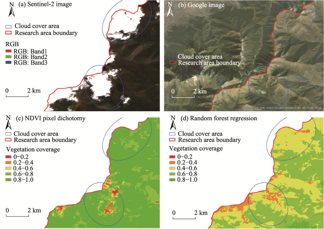
Fig. 8 Comparison of inversion results of the random forest regression model and the NDVI pixel dichotomy model in cloud cover areas |
This research is supported by “The National Science and Technology Major Project of the Ministry of Science and Technology of China”. The authors would like to thank the editors and anonymous reviewers for their useful comments in improving the article. We would like to thank the PhoREAL team and Google earth engine team for their support of the ICESat-2, Sentinel-1, Sentinel-2 and landuse data processing aspects. We are very grateful for the NASA and the Alaska Satellite Facility for distributing the ICESat-2 data (
| [1] |
|
| [2] |
|
| [3] |
|
| [4] |
|
| [5] |
|
| [6] |
|
| [7] |
|
| [8] |
|
| [9] |
|
| [10] |
|
| [11] |
|
| [12] |
|
| [13] |
|
| [14] |
|
| [15] |
|
| [16] |
|
| [17] |
|
| [18] |
|
| [19] |
|
| [20] |
|
| [21] |
|
| [22] |
|
| [23] |
|
| [24] |
|
| [25] |
|
/
| 〈 |
|
〉 |
