
Journal of Resources and Ecology >
Spatial and Temporal Differentiation Trends and Attributions of High-quality Development in the Huaihe Eco-economic Belt
Received date: 2022-04-13
Accepted date: 2022-08-12
Online published: 2023-04-21
Supported by
The University Scientific Research Key Project(SK2021A0402)
The University Scientific Research Key Project(SK2021A0413)
The Talents Support Project(2022KYQD008)
The College Students Innovation and Entrepreneurship Training Program(202110371018)
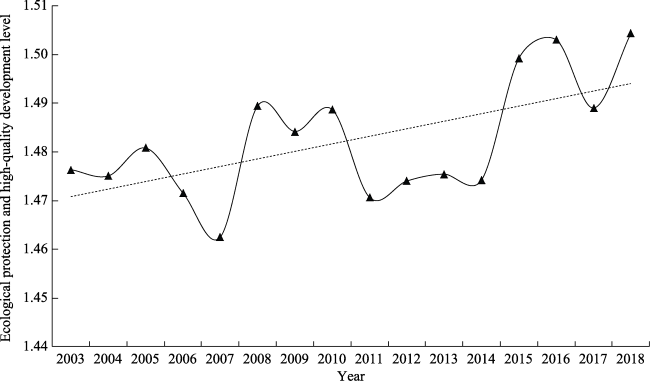
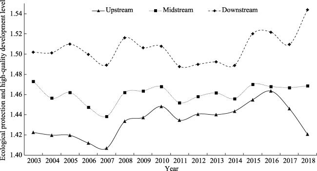
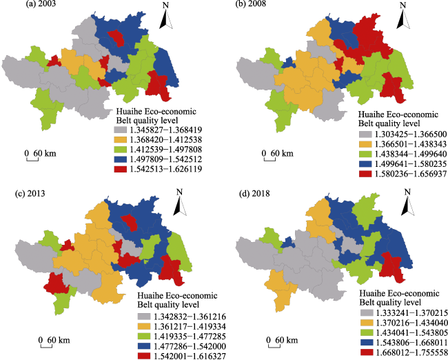
The Huaihe River Basin is one of the typical large river basin economies, promoting its ecological protection and high-quality development is a strategic choice to improve the quality of China’s economic development and narrow the regional development gap, which has far-reaching strategic value for the region and the country in the new era. Based on the theoretical connotation of watershed ecological protection and high-quality economic development, starting from the special characteristics and practical features of the Huaihe River Eco-economic Belt, the panel data of 28 prefecture-level cities in the Huaihe River Eco-economic Belt from 2003-2018 are used as the research samples, the improved entropy method, Dagum Gini coefficient method and panel Tobit model investigate and analyze the time and space of ecological protection and high-quality development in the Huaihe Eco-economic Belt Evolution characteristics and promotion drivers. The results show that the overall ecological protection and high-quality development level of the Huaihe River Eco-economic Belt is 1.4824, showing an overall upward trend, with obvious periodic fluctuations; the high-value areas are mainly located in the lower and middle reaches of the basin, with the spatial agglomeration characteristic of “double core leading”, while the upper reaches are always in the stage of “low level and stable growth trap”; the hypervariable density is the main cause of the regional disparity; per capita output, opening to the outside world, human capital and government intervention drive the improvement of ecological protection and high-quality development. There are significant differences in the driving factors of ecological protection and high-quality development in the upper, middle and lower reaches of the city. The study of the development status of the Huaihe River Eco-economic Belt and its evolution law are of great theoretical significance, practical value for analyzing the synergistic enhancement path of urban ecological protection and high-quality development, promoting the ecological protection and high-quality economic development of the entire Huaihe River Basin.
CHENG Yongsheng , ZHANG Deyuan . Spatial and Temporal Differentiation Trends and Attributions of High-quality Development in the Huaihe Eco-economic Belt[J]. Journal of Resources and Ecology, 2023 , 14(3) : 517 -532 . DOI: 10.5814/j.issn.1674-764x.2023.03.008
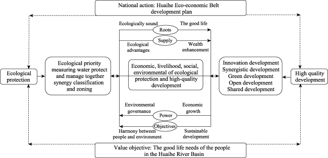
Fig. 1 The mechanism of the role of ecological protection and high-quality development in the Huaihe Eco-economic Belt |
Table 1 Urban scope of the Huaihe Eco-economic Belt |
| Region | City quantity | Huaihe Eco-economic Belt Cities |
|---|---|---|
| Upstream | 9 | Xinyang City, Zhumadian City, Zhoukou City, Luohe City, Shangqiu City, Pingdingshan City, Nanyang City, Suizhou City, Xiaogan City |
| Midstream | 8 | Bengbu City, Huainan City, Fuyang City, Lu’an City, Bozhou City, Suzhou City, Huaibei City, Chuzhou City |
| Downstream | 11 | Huaian City, Yancheng City, Suqian City, Xuzhou City, Lianyungang City, Yangzhou City, Taizhou City, Zaozhuang City, Jining City, Linyi City, Heze City |
Table 2 Comprehensive evaluation index system of ecological protection and high-quality development level |
| Target layer | Criterion layer | Indicator layer | Indicator properties |
|---|---|---|---|
| Ecological protection and high-quality development level | Economic and ecological protection and high-quality development | GDP per capita | + |
| Fixed asset investment per unit of GDP | + | ||
| The proportion of secondary industry | + | ||
| The proportion of the tertiary industry | + | ||
| Disposable income per capita | + | ||
| Domestic electricity consumption per capita | + | ||
| Ecological protection of people’s livelihood and high-quality development | Proportion of urban population | + | |
| Density of population | + | ||
| Every 100000 college students | + | ||
| Urban registered unemployment rate | - | ||
| The proportion of employees in the secondary industry | + | ||
| The proportion of employees in the tertiary industry | + | ||
| Consumption expenditure per capita | + | ||
| Social and ecological protection and high-quality development | Road area per capita | + | |
| Public transportation per 10000 people | + | ||
| Library collection per hundred people | + | ||
| LPG penetration rate | + | ||
| Beds per thousand population | + | ||
| Environmental protection and high-quality development | Industrial wastewater discharge | - | |
| Industrial SO2 Emissions | - | ||
| Industrial smoke (dust) emissions | - | ||
| Comprehensive utilization rate of industrial solid waste | + | ||
| Wastewater discharge compliance rate | + | ||
| Green area per capita | + | ||
| Green coverage in built- up areas | + |
Note: “+” refers to positive indicators, “-” refers to negative indicators. |
Table 3 The measurement results of ecological protection and high-quality development in the Huaihe Economic Belt |
| City | Ecological protection and high-quality development level | City | Ecological protection and high-quality development level |
|---|---|---|---|
| Yangzhou | 1.641 | Chuzhou | 1.500 |
| Taizhou | 1.611 | Pingdingshan | 1.477 |
| Huaibei | 1.588 | Xiaogan | 1.460 |
| Xuzhou | 1.583 | Suqian | 1.451 |
| Zaozhuang | 1.571 | Fuyang | 1.420 |
| Luohe | 1.565 | Zhumadian | 1.394 |
| Jining | 1.557 | Zhoukou | 1.394 |
| Bengbu | 1.553 | Heze | 1.393 |
| Lianyungang | 1.551 | Bozhou | 1.388 |
| Linyi | 1.546 | Shangqiu | 1.385 |
| Huainan | 1.528 | Suzhou | 1.368 |
| Suizhou | 1.511 | Nanyang | 1.360 |
| Huaian | 1.510 | Xinyang | 1.359 |
| Yancheng | 1.502 | Lu’an | 1.341 |
Fig. 2 Dynamic trend of the overall ecological protection and high-quality development level of the Huaihe Eco-economic Belt |
Fig. 3 Dynamic trend of ecological protection and high-quality development levels in the three major regions |
Fig. 4 Spatial distribution of ecological protection and high-quality development levels |
Table 4 The regional gap between ecological protection and high-quality development and its source breakdown |
| Year | Overall regional disparity | Intra-regional disparity | Regional disparity | Hypervariable density | Contribution rate (%) | ||
|---|---|---|---|---|---|---|---|
| Intra-regional disparity | Regional disparity | Hypervariable density | |||||
| 2003 | 0.0340 | 0.0093 | 0.0053 | 0.0194 | 27.35 | 15.59 | 57.06 |
| 2004 | 0.0379 | 0.0107 | 0.0063 | 0.0209 | 28.23 | 16.62 | 55.15 |
| 2005 | 0.0372 | 0.0100 | 0.0093 | 0.0179 | 26.88 | 25.00 | 48.12 |
| 2006 | 0.0360 | 0.0091 | 0.0089 | 0.0180 | 25.28 | 24.72 | 50.00 |
| 2007 | 0.0351 | 0.0092 | 0.0080 | 0.0179 | 26.21 | 22.79 | 51.00 |
| 2008 | 0.0358 | 0.0093 | 0.0097 | 0.0168 | 25.98 | 27.09 | 46.93 |
| 2009 | 0.0320 | 0.0089 | 0.0072 | 0.0159 | 27.81 | 22.50 | 49.69 |
| 2010 | 0.0314 | 0.0090 | 0.0058 | 0.0166 | 28.66 | 18.47 | 52.87 |
| 2011 | 0.0314 | 0.0092 | 0.0055 | 0.0167 | 29.30 | 17.52 | 53.18 |
| 2012 | 0.0311 | 0.0093 | 0.0038 | 0.0180 | 29.90 | 12.22 | 57.88 |
| 2013 | 0.0320 | 0.0094 | 0.0044 | 0.0182 | 29.38 | 13.75 | 56.88 |
| 2014 | 0.0306 | 0.0090 | 0.0043 | 0.0173 | 29.41 | 14.05 | 56.54 |
| 2015 | 0.0354 | 0.0098 | 0.0079 | 0.0177 | 27.68 | 22.32 | 50.00 |
| 2016 | 0.0375 | 0.0104 | 0.0075 | 0.0196 | 27.73 | 20.00 | 52.27 |
| 2017 | 0.0343 | 0.0097 | 0.0062 | 0.0184 | 28.28 | 18.08 | 53.64 |
| 2018 | 0.0482 | 0.0122 | 0.0153 | 0.0207 | 25.31 | 31.74 | 42.95 |
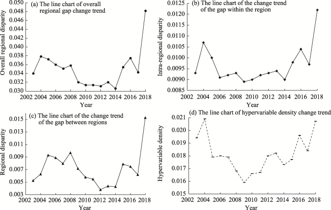
Fig. 5 Dynamic trends of regional gaps in ecological protection and high-quality development (a) The line chart of overall regional gap change trend; (b) The line chart of the change trend of the gap within the region; (c) The line chart of the change trend of the gap between regions; (d) The line chart of hypervariable density change trend |
Table 5 Descriptive statistics of related variables (N=448) |
| Variable (unit) | Minimum | Maximum | Mean | Standard deviation |
|---|---|---|---|---|
| Pgdp (10000 yuan) | 0.2611 | 6.9004 | 1.858 | 1.1977 |
| Pgdp2 (10000 yuan) | 0.0682 | 47.6157 | 4.8834 | 6.3949 |
| Open (%) | 0.1889 | 18.6157 | 2.2862 | 2.1389 |
| Hum (yr) | 7.8852 | 10.4262 | 8.9768 | 0.4817 |
| Gov (%) | 0.0596 | 1.4852 | 0.1489 | 0.0875 |
| Tech (Pcs/10000) | 0.0508 | 49.6819 | 3.2082 | 5.2775 |
| Reg (-) | 0.0004 | 1.0150 | 0.0717 | 0.1236 |
Table 6 Model estimation results |
| Independent variable | Dependent variable | |||||||||
|---|---|---|---|---|---|---|---|---|---|---|
| Full sample | The full sample with one period lag | Upstream | Midstream | Downstream | ||||||
| OLS | Tobit | OLS | Tobit | OLS | Tobit | OLS | Tobit | OLS | Tobit | |
| Pgdp | 0.000*** | 0.000*** | 0.000*** | 0.000*** | 0.002*** | 0.002*** | 0.000*** | 0.000*** | 0.031** | 0.016** |
| (0.0106) | (0.0085) | (0.0105) | (0.0092) | (0.0242) | (0.0241) | (0.0395) | (0.0348) | (0.0116) | (0.0103) | |
| Pgdp2 | 0.909 | 0.885 | 0.773 | 0.735 | 0.748 | 0.749 | 0.002** | 0.001*** | 0.322 | 0.322 |
| (0.0024) | (0.0019) | (0.0025) | (0.0021) | (0.0074) | (0.0075) | (0.0078) | (0.0075) | (0.0020) | (0.0020) | |
| Open | 0.000*** | 0.000*** | 0.009*** | 0.000*** | 0.016** | 0.016** | 0.216 | 0.31 | 0.002*** | 0.002*** |
| (0.0019) | (0.0015) | (0.0023) | (0.0015) | (0.0033) | (0.0033) | (0.0022) | (0.0027) | (0.0024) | (0.0024) | |
| Hum | 0.000*** | 0.000*** | 0.000*** | 0.000*** | 0.000*** | 0.000*** | 0.796 | 0.771 | 0.000*** | 0.000*** |
| (0.0113) | (0.0070) | (0.0111) | (0.0071) | (0.0112) | (0.0130) | (0.0192) | (0.0170) | (0.0103) | (0.0106) | |
| Gov | 0.069* | 0.000*** | 0.043** | 0.000*** | 0.000*** | 0.000*** | 0.000*** | 0.000*** | 0.113 | 0.001*** |
| (0.1551) | (0.0337) | (0.1451) | (0.0340) | (0.1249) | (0.1236) | (0.0959) | (0.0971) | (0.0711) | (0.0344) | |
| Tech | 0.494 | 0.453 | 0.482 | 0.45 | 0.125 | 0.198 | 0.236 | 0.332 | 0.028** | 0.082* |
| (0.0012) | (0.0011) | (0.0014) | (0.0013) | (0.0103) | (0.0122) | (0.0030) | (0.0037) | (0.0008) | (0.0010) | |
| Reg | 0.227 | 0.137 | 0.211 | 0.119 | 0.496 | 0.602 | 0.193 | 0.151 | 0.106 | 0.026** |
| (0.0293) | (0.0238) | (0.0296) | (0.0237) | (0.0739) | (0.0966) | (0.0349) | (0.0316) | (0.1289) | (0.0929) | |
| Constant term | 0.000*** | 0.000*** | 0.000*** | 0.000*** | 0.000*** | 0.000*** | 0.000*** | 0.000*** | 0.000*** | 0.000*** |
| (0.1106) | (0.0608) | (0.1072) | (0.0620) | (0.0973) | (0.1144) | (0.1623) | (0.1475) | (0.0976) | (0.0963) | |
| Observations | 448 | 448 | 420 | 420 | 144 | 144 | 128 | 128 | 176 | 176 |
Note: *, ** and *** represent the significance levels of 10%, 5% and 1%, respectively, and the numbers in parentheses of the model represent standard errors. |
| [1] |
|
| [2] |
|
| [3] |
|
| [4] |
|
| [5] |
|
| [6] |
|
| [7] |
|
| [8] |
|
| [9] |
|
| [10] |
|
| [11] |
|
| [12] |
|
| [13] |
|
| [14] |
|
| [15] |
|
| [16] |
|
| [17] |
|
| [18] |
|
/
| 〈 |
|
〉 |