
Journal of Resources and Ecology >
Market-incentive Environmental Regulation and Urban Resilience: Heterogeneity and Influence Mechanisms
Received date: 2022-01-10
Accepted date: 2022-07-20
Online published: 2023-04-21
Supported by
The National Natural Science Foundation of China Youth Project(72103113)
The Humanities and Social Science Fund of Ministry of Education of China(21YJA630071)
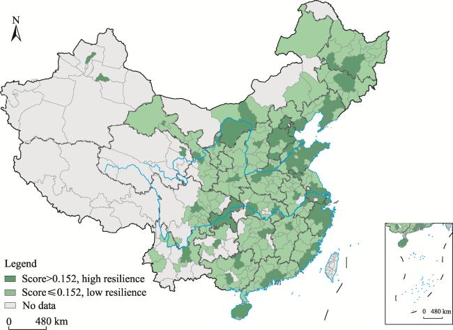
The market-incentive emission trading system is an important element for improving urban governance. The main objective of this study was to examine the hypothesis that market-incentive environmental regulations have an impact on urban resilience. The entropy method was used to construct six dimension-specific objectives to comprehensively portray the level of urban resilience, and then the double difference method and the moderation model were used to investigate the impact of market-incentive environmental regulation on urban resilience and its mechanisms. The results show that up to two-thirds of cities are at a low resilience level. Second, the emission trading system significantly enhances the resilience of cities over time. Moreover, the effects of energy saving and emission reduction, marketization level and innovation vitality are important mechanisms for improving the resilience of cities. Furthermore, the lower the degree of green development of the city itself, the more significant the effect of the emission trading system on improving the resilience of the city. For different types of resource-based cities, the enhancement effects on urban resilience are growth cities, regeneration cities, mature cities and declining cities in descending order. To improve the level of urban resilience, it is necessary to release the policy dividend of regional coordination and to deepen development according to regional endowment differences. Finally, the findings of this analysis can provide some theoretical support and experience reference for deepening the market-incentive reform of environmental governance and promoting the high-quality development of resilient cities.
LIU Yaqin , LI Min . Market-incentive Environmental Regulation and Urban Resilience: Heterogeneity and Influence Mechanisms[J]. Journal of Resources and Ecology, 2023 , 14(3) : 502 -516 . DOI: 10.5814/j.issn.1674-764x.2023.03.007
Table 1 Evaluation index system of urban resilience in China |
| Goal level | Subsystem level | Weight (%) | Index level | Weight (%) | Attribute |
|---|---|---|---|---|---|
| Urban resilience level | Economy | 23.46 | Industrial structure sophistication | 0.59 | + |
| Industrial structure rationalization | 10.51 | + | |||
| Per capita savings | 7.37 | + | |||
| Per capita gross regional product | 4.99 | + | |||
| Society | 8.57 | Urban unemployment rate | 0.06 | - | |
| Population density | 0.21 | - | |||
| Number of health practitioners per 1000 people | 2.63 | + | |||
| Mobile phone penetration rate | 5.66 | + | |||
| Infrastructure | 31.87 | Road area per capita | 3.39 | + | |
| Number of public transport per 10000 people | 3.69 | + | |||
| Water availability and supply capacity | 3.64 | + | |||
| Energy poverty indicators | 8.08 | + | |||
| Coverage rate of medical institutions | 5.81 | + | |||
| Coverage rate of medical beds | 7.25 | + | |||
| Ecology | 9.98 | Wastewater emissions | 0.40 | - | |
| Waste gas emissions | 0.64 | - | |||
| Smoke emissions | 0.39 | - | |||
| Comprehensive utilization rate of solid waste | 1.32 | + | |||
| Wastewater disposal rate | 1.51 | + | |||
| Waste disposal rate | 1.08 | + | |||
| Greening coverage | 0.88 | + | |||
| Sulfur dioxide removal rate | 3.75 | + | |||
| Community | 2.79 | Proportion of social service workers | 2.79 | + | |
| Institution | 23.35 | Basic medical insurance rate | 11.27 | + | |
| Unemployment insurance rate | 12.08 | + |
Fig. 1 Distribution of urban resilience in China |
Table 2 Descriptive statistics of the main variables |
| Variable | Symbol | Computing method | Sample size | Mean | Standard deviation |
|---|---|---|---|---|---|
| Urban resilience | score | Index system constructed by the entropy weight method | 4544 | 0.152 | 0.072 |
| Industrial structure | ind | Proportion of total industrial output value above the limit to GDP | 4544 | 0.069 | 0.039 |
| R&D and innovation capacity | fintio | Proportion of expenditure on science and education | 4544 | 0.093 | 0.028 |
| Energy supply | pow | Gas and natural gas supply | 4528 | 0.065 | 0.129 |
| Research and innovation vitality | scitio | Proportion of research personnel | 4544 | 0.048 | 0.075 |
| Environmental protection awareness | envitio | Number of people engaged in environmental protection divided by the total number of people | 4544 | 0.111 | 0.089 |
| Land-use planning | areaio | Proportion of urban construction land in the urban area (%) | 4544 | 0.182 | 0.199 |
Table 3 Basic regression results |
| Variable | Average treatment effect | Dynamic effect |
|---|---|---|
| did | 0.105*** (0.007) | |
| treated×year2007 | 0.024** (0.040) | |
| treated×year2008 | 0.040** (0.018) | |
| treated×year2009 | 0.072*** (0.009) | |
| treated×year2010 | 0.060*** (0.008) | |
| treated×year2011 | 0.050*** (0.006) | |
| treated×year2012 | 0.048*** (0.002) | |
| treated×year2013 | 0.072*** (0.003) | |
| treated×year2014 | 0.098*** (0.001) | |
| treated×year2015 | 0.069*** (0.001) | |
| treated×year2016 | 0.074*** (0.006) | |
| treated×year2017 | 0.087*** (0.008) | |
| treated×year2018 | 0.106*** (0.008) | |
| Control variables | Yes | Yes |
| Time effects | Yes | Yes |
| Individual city effects | Yes | Yes |
| Province effects | Yes | Yes |
| Adjusted R2 | 0.847 | 0.847 |
| N | 4528 | 4528 |
Notes: ***, ** denote the 1% and 5% significance levels, respectively. All estimates control for city and year fixed effects, N is the number of samples. The did stands for the core explanatory variable. The value of a pilot city implementing an emission trading policy is 1, otherwise it is 0. The numbers in parentheses are P values. |
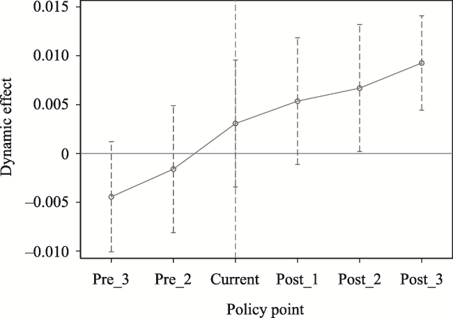
Fig. 2 Dynamic effect of the parallel trend hypothesis |
Table 4 Excluding the regression results of energy policy |
| Variable | Average treatment effect | Dynamic effect |
|---|---|---|
| did | 0.121*** (0.000) | |
| treated×year2007 | 0.016*** (0.008) | |
| treated×year2008 | 0.030*** (0.000) | |
| treated×year2009 | 0.062*** (0.000) | |
| treated×year2010 | 0.051*** (0.000) | |
| treated×year2011 | 0.041*** (0.000) | |
| treated×year2012 | 0.039*** (0.000) | |
| treated×year2013 | 0.062*** (0.000) | |
| treated×year2014 | 0.088*** (0.000) | |
| treated×year2015 | 0.060*** (0.000) | |
| treated×year2016 | 0.066*** (0.000) | |
| treated×year2017 | 0.079*** (0.000) | |
| treated×year2018 | 0.098*** (0.000) | |
| Control variables | Yes | Yes |
| Time effects | Yes | Yes |
| Individual city effects | Yes | Yes |
| Province effects | Yes | Yes |
| Adjusted R2 | 0.843 | 0.843 |
| N | 2688 | 2688 |
Notes: *** denotes the 1% significance level. All estimates control for city and year fixed effects, and N is the number of samples. The numbers in parentheses are P values. |
Table 5 PSM balance test |
| Covariates | Mean | Standard deviation (%) | Error reduction (%) | T-test | |||
|---|---|---|---|---|---|---|---|
| Experimental groups | Control groups | t | P | ||||
| gdpfin | Before matching | 0.082 | 0.103 | -33.400 | -10.430 | 0.000 | |
| After matching | 0.084 | 0.085 | -1.500 | 95.600 | -0.550 | 0.585 | |
| gindtio | Before matching | 0.070 | 0.068 | 5.300 | 1.700 | 0.090 | |
| After matching | 0.071 | 0.071 | -0.400 | 92.800 | -0.120 | 0.905 | |
| high | Before matching | 0.607 | 0.549 | 40.500 | 13.060 | 0.000 | |
| After matching | 0.603 | 0.603 | -0.300 | 99.300 | -0.090 | 0.932 | |
| so2emil | Before matching | 0.746 | 0.831 | -43.700 | -14.830 | 0.000 | |
| After matching | 0.775 | 0.779 | -2.300 | 94.700 | -0.710 | 0.476 | |
| rational | Before matching | 0.047 | 0.041 | 9.200 | 3.070 | 0.002 | |
| After matching | 0.044 | 0.044 | 0.000 | 99.800 | -0.010 | 0.996 | |
| gdpper | Before matching | 0.286 | 0.258 | 12.700 | 4.160 | 0.000 | |
| After matching | 0.279 | 0.283 | -1.600 | 87.300 | -0.460 | 0.644 | |
| ind | Before matching | 0.177 | 0.118 | 30.700 | 10.340 | 0.000 | |
| After matching | 0.161 | 0.162 | -0.100 | 99.700 | -0.030 | 0.978 | |
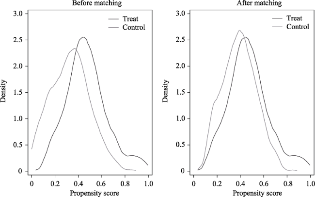
Fig. 3 PSM common support hypothesis test |
Table 6 Robust regression results |
| Variable | Average treatment effect | Dynamic effect | Variable | Average treatment effect | Dynamic effect |
|---|---|---|---|---|---|
| did | 0.005*** (0.000) | treated×year2014 | 0.088** (0.018) | ||
| treated×year2007 | 0.023* (0.081) | treated×year2015 | 0.077** (0.025) | ||
| treated×year2008 | 0.031* | treated×year2016 | 0.086** (0.040) | ||
| (0.072) | |||||
| treated×year2009 | 0.040* | treated×year2017 | 0.093** (0.036) | ||
| (0.056) | |||||
| treated×year2010 | 0.052** | treated×year2018 | 0.099** (0.034) | ||
| (0.041) | |||||
| treated×year2011 | 0.056** (0.022) | Control variables | Yes | Yes | |
| Time effects | Yes | Yes | |||
| treated×year2012 | 0.073** (0.016) | Individual city effects | Yes | Yes | |
| Province effects | No | No | |||
| treated×year2013 | 0.071** (0.020) | Adjusted R2 | 0.774 | 0.773 | |
| N | 4027 | 4027 |
Notes: ***, ** and * denote the 1%, 5% and 10% significance levels, respectively. All estimates control for city and year fixed effects, and N is the number of samples. The numbers in parentheses are P values. |
Table 7 Test of the influence mechanism |
| Variable | Energy utilization efficiency | Marketization index | Innovation vitality |
|---|---|---|---|
| did×Adv | 0.109*** (0.005) | 0.040** (0.014) | 0.008** (0.036) |
| Adv | 0.005 (0.972) | 0.138*** (0.007) | 0.794*** (0.003) |
| Control variables | Yes | Yes | Yes |
| Time effects | Yes | Yes | Yes |
| Individual city effects | Yes | Yes | Yes |
| Province effects | No | No | No |
| Adjusted R2 | 0.731 | 0.445 | 0.642 |
| N | 4528 | 4544 | 4544 |
Note: ***, ** denote the 1% and 5% significance levels, respectively. All estimates control for city and year fixed effects, and N is the number of samples. The numbers in parentheses are P values. |
Table 8 Heterogeneity analysis of the green development level |
| Variable | Average treatment effect | Dynamic effect |
|---|---|---|
| did | 0.019*** (0.000) | |
| treated×year2007 | 0.019*** (0.000) | |
| treated×year2008 | 0.024*** (0.000) | |
| treated×year2009 | 0.033*** (0.000) | |
| treated×year2010 | 0.041*** (0.000) | |
| treated×year2011 | 0.045*** (0.000) | |
| treated×year2012 | 0.060*** (0.000) | |
| treated×year2013 | 0.057*** (0.000) | |
| treated×year2014 | 0.074*** (0.000) | |
| treated×year2015 | 0.064*** (0.000) | |
| treated×year2016 | 0.071*** (0.000) | |
| treated×year2017 | 0.079*** (0.000) | |
| treated×year2018 | 0.088*** (0.000) | |
| Control variables | Yes | Yes |
| Time effects | Yes | Yes |
| Individual city effects | Yes | Yes |
| Province effects | No | No |
| Adjusted R2 | 0.771 | 0.757 |
| N | 1856 | 1856 |
Note: *** denotes the 1% significance level. All estimates control for city and year fixed effects, and N is the number of samples. The numbers in parentheses are P values. |
Table 9 Heterogeneity analysis of resource endowment |
| Variable | Total sample | Growing | Mature | Declining | Regenerative |
|---|---|---|---|---|---|
| did | 0.014*** (0.000) | 0.022* (0.071) | 0.012*** (0.000) | 0.001 (0.836) | 0.019** (0.028) |
| Control variables | Yes | Yes | Yes | Yes | Yes |
| Time effects | Yes | Yes | Yes | Yes | Yes |
| Individual city effects | Yes | Yes | Yes | Yes | Yes |
| Province effects | No | No | No | No | No |
| Adjusted R2 | 0.832 | 0.808 | 0.868 | 0.852 | 0.79 |
| N | 1824 | 224 | 992 | 368 | 240 |
Note: ***, ** and * denote the 1%, 5% and 10% significance levels, respectively. All estimates control for city and year fixed effects, and N is the number of samples. The numbers in parentheses are P values. |
| [1] |
|
| [2] |
|
| [3] |
|
| [4] |
|
| [5] |
|
| [6] |
|
| [7] |
|
| [8] |
|
| [9] |
|
| [10] |
|
| [11] |
|
| [12] |
|
| [13] |
|
| [14] |
|
| [15] |
|
| [16] |
|
| [17] |
|
| [18] |
|
| [19] |
|
| [20] |
|
| [21] |
|
| [22] |
|
| [23] |
|
| [24] |
|
| [25] |
|
| [26] |
|
| [27] |
|
| [28] |
|
| [29] |
|
| [30] |
|
| [31] |
|
| [32] |
|
| [33] |
|
| [34] |
|
| [35] |
|
| [36] |
|
| [37] |
|
| [38] |
|
| [39] |
|
| [40] |
|
| [41] |
|
| [42] |
|
| [43] |
|
| [44] |
|
| [45] |
|
| [46] |
|
| [47] |
|
| [48] |
|
| [49] |
|
| [50] |
|
| [51] |
|
| [52] |
|
| [53] |
|
| [54] |
|
| [55] |
|
| [56] |
|
| [57] |
|
/
| 〈 |
|
〉 |