Carbon Emissions

The Spatial-temporal Characteristics of PM2.5 Concentrations in Chinese Cities and the Influencing Factors

  • LIU Qingqing , 1 ,
  • YU Hu , 2, * ,
  • ZHANG Pengfei 3 ,
  • LUO Qing 4
Expand
  • 1. College of Tourism and Exhibition, Henan University of Economics and Law, Zhengzhou 450046, China
  • 2. Institute of Geographic Sciences and Natural Resources Research, Chinese Academy of Sciences, Beijing 100101, China
  • 3. School of Economic Management, Yanshan University, Qinhuangdao, Hebei 066004, China
  • 4. College of Resources and Environment, Henan University of Economics and Law, Zhengzhou 450046, China
*YU Hu, E-mail:

LIU Qingqing, E-mail:

Received date: 2021-12-23

  Accepted date: 2022-07-19

  Online published: 2023-04-21

Supported by

The Strategic Pilot Science and Technology Project of the Chinese Academy of Sciences (Class A)(XDA20020302)

The Key Research and Development Project of Xinjiang Autonomous Region(2021B03002-2)

Abstract

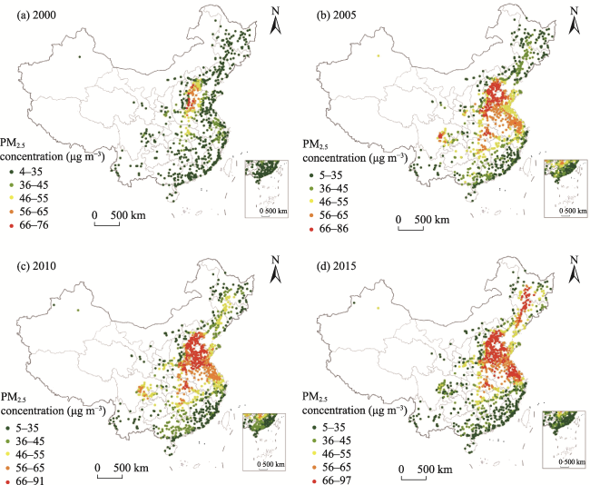
Based on the scientific identification of urban built-up areas, the spatial and temporal characteristics of PM2.5 concentrations in Chinese cities during 2000-2015, and the factors influencing them, were analyzed by exploratory spatial analysis and spatial econometric models. The results showed that the concentration of PM2.5 in Chinese cities increased in an inverted “L” pattern during 2000-2015. However, the cities with high PM2.5 concentrations are characterized by large-scale agglomeration, and urban agglomeration is an urban agglomeration area with a high PM2.5 concentration. Specifically, the areas with high PM2.5 concentrations are affected by natural factors, social and economic factors and urban form factors which all work together. From 2000 to 2005, the annual average concentration of PM2.5 across all Chinese cities increased from 31.19 μg m-³ to 46.00 μg m-³, and small-scale high concentrations were densely concentrated at the intersection of Hebei, Shandong and Henan. From 2005 to 2010 and from 2010 to 2015, the annual average growth rate of the PM2.5 concentration in urban areas slowed down, with average levels of 47.67 μg m-³ in 2010 and 48.72 μg m-³ in 2015, representing increases of only 3.63% and 2.20%, respectively. In 2010, the high-concentration agglomeration areas expanded to include the Beijing-Tianjin-Hebei region, the Central Yangtze River, the Yangtze River Delta, and the Chengdu Plain; while in 2015 they further expanded to the entire North China Plain, the Central Yangtze River, and the Harbin-Changchun region.

Cite this article

LIU Qingqing , YU Hu , ZHANG Pengfei , LUO Qing . The Spatial-temporal Characteristics of PM2.5 Concentrations in Chinese Cities and the Influencing Factors[J]. Journal of Resources and Ecology, 2023 , 14(3) : 433 -444 . DOI: 10.5814/j.issn.1674-764x.2023.03.001

1 Introduction

In the past decade, with the rapid advancement of urbanization and increase in energy consumption, the average concentration of PM2.5 in Chinese cities increased from 31.19 μg m-3 in 2000 to 48.72 μg m-3 in 2015, representing an increase of 55.24% in 15 years. Especially since 2013, most cities in central and eastern China have experienced frequent hazy weather every winter. Urban air pollution in China has led to serious health consequences and socioeconomic impacts (Yan et al., 2019). According to the 2016 Global Air Quality Report of the World Health Organization, nearly 2 million people in China die every year from pollution caused by fine particles in the environment and indoor air. Among them, half of the deaths are caused by environmental air pollution. An Organization for Economic Co-operation and Development (OECD) study found that in the 21st century, China’s environmental pollution is closely related to its rapid economic development (Li et al., 2018). In this context, the prevention and control of PM2.5 pollution have become a major focus of attention for Chinese governments at all levels, academia, and ordinary people.
The prevention and control of fine particulate matter (PM2.5) require an accurate understanding of its temporal and spatial evolutionary trends and the factors driving those trends. Many studies have examined the temporal and spatial evolution of PM2.5 concentrations in China and their causes (Beckett et al., 2000; Yuan et al., 2019). Some studies have shown that PM2.5 concentrations in China have been reduced due to the implementation of emission reduction measures (Zhang et al., 2018), while other studies have shown that China’s PM2.5 concentrations have increased, and the range of high concentrations has continued to expand. Related research uses data from different sources, such as remote sensing and ground monitoring stations, to reveal the temporal and spatial distribution characteristics of PM2.5 pollution at different temporal and spatial scales (Ma et al., 2019). However, the research results for a given region and a given time period will also vary, which is largely related to differences in the data sources, time scales and spatial scales among different studies. On the whole, with the availability of more refined data, research on the temporal and spatial evolution of PM2.5 concentrations has shown a transition from a macro scale to a micro scale. At the same time, the study scope has also changed from a single city or city cluster to a larger area.
The urban PM2.5 concentration is affected by natural conditions, social economy, urban form and structure, and other factors. Some studies emphasize the relationship between geographical conditions and the urban PM2.5 concentration, such as temperature, rainfall, wind speed and other meteorological conditions, topographic features, and vegetation coverage (Yang et al., 2020). Also, rainfall and wind speed have a diluting effect on the PM2.5 concentration (Wang et al., 2018). The terrain of a piedmont plain severely hinders the horizontal flow and vertical exchange of air and the vegetation coverage will have a positive effect of decreasing the urban PM2.5 concentration (Yang et al., 2020). Other studies have emphasized the impacts of economic development, energy consumption, and economic structure on air quality (Boone et al., 2014). Research has also suggested that economic development, urbanization and haze pollution are related, and that there is an impact of economic agglomeration on improving energy efficiency and reducing pollution, and an impact of industrial structural evolution on PM2.5 emissions (Wang et al., 2018). Furthermore, researchers have found that the urban form will affect the PM2.5 concentration through vehicles, green space control, and greenhouse gas emissions (Yuan et al., 2019). Notably, the size of the impact is related to the type and scale of the city (Ewing and Cervero, 2010; Hankey and Marshall, 2010; Lee, 2020). In the absence of efficient transportation systems, the decentralized expansion of cities will lead to longer commuting distances, in turn leading to serious air quality problems (Yan et al., 2019). However, the strength of the relationship between urban form and air quality will vary with the level of economic development and city size (McCarty and Kaza, 2015; Zhang et al., 2018). The city’s plan shape, functional structure, land use types, and other attributes will also affect the residents’ commuting distances and commuting patterns, which in turn affect urban energy consumption and air pollutant emissions (Yuan et al., 2019).
Existing studies are mainly based on cross-sectional data, and focus on the influences of special factors. Comprehensive research on different influencing factors is still relatively weak, and the interaction mechanisms between the PM2.5 concentration and its influencing factors are relatively complex, with considerable uncertainty. At the same time, although the PM2.5 concentration will have significant variation over a small range, few studies have considered it from the urban area scale. As urban areas have relatively high PM2.5 concentrations, the three research questions raised in this study are:
What are the characteristics of the temporal and spatial distributions of PM2.5 concentrations in urban areas?
What are the roles of natural factors, socio-economic factors, and urban form and structure in causing the differences in urban PM2.5 concentrations?
Over time, how have the magnitudes and directions of these factors changed?
Only by clarifying these issues can we more effectively prevent and control urban PM2.5. Given that the PM2.5 concentrations in urban areas are significantly higher than those in the surrounding areas (Yang et al., 2020), this paper combines land use and population density data and analyzes the urban PM2.5 based on identifying urban areas in China from 2000 to 2015. Exploring the temporal and spatial evolutionary characteristics of the concentrations and their influencing factors will provide a decision-making reference for urban PM2.5 pollution prevention and control and the development of healthy cities.
This study explores the spatial-temporal characteristics and factors influencing PM2.5 concentrations at the national scale, and clearly delineates the PM2.5 concentration changes in major regions such as the Yangtze River Delta urban agglomeration, the North China Plain, and the Pearl River Delta urban agglomeration. Studying PM2.5 concentration changes from a spatial-temporal perspective can improve the research framework of air pollution in general, and enrich the relevant research results of atmospheric environmental changes in China. At the same time, 2000-2015 was a period of rapid economic development in China, so exploring the changes in PM2.5 concentrations can verify the interactive relationship between economic development and air pollution. As the research results show, the spatial-temporal distribution of PM2.5 concentrations in Chinese cities is a result of the comprehensive effects of natural factors, social and economic factors, urban form and other factors, which provides a theoretical basis for optimizing the developmental relationship between urban economy and air pollution.

2 Research methods

2.1 Identification of urban areas

Following the method proposed by GRUMP, this study uses a 1 km×1 km grid as the basic spatial unit and identifies adjacent grids with population densities greater than 1500 people km-2 or with construction land ratios of more than 50% and total areas of more than 10 km2 as the central cities (Center for International Earth Science Information Network, 2004). The specific identification steps are as follows: 1) Filter out all grids with a population density greater than 1500 people km-2 and grids with a construction land ratio greater than 50%, and superimposing the two; 2) Combine adjacent grids and select the patches with an area greater than 10 km2 as urban areas; 3) Fill the blank grids in the urban areas and smooth the edges using an iterative method (Fig. 1). In other words, each grid has eight surrounding grids and if more than five of the eight are high-density grids, then that center grid will be filled in as a high-density grid and added to the high-density agglomeration area. This operation was repeated until no more grids were added. The built-up urban areas identified according to the above criteria may exist in the scope of the city but beyond the municipal area, or beyond the scope of the city but connected to other urban built-up areas, and the spatial separation of multiple urban built-up areas within a city often occurs.
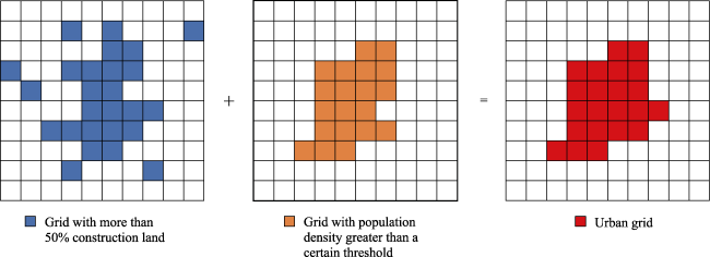
Fig. 1 The process of urban area identification

2.2 Spatial measurement model

The premise of the general linear regression model estimated by the ordinary least squares (OLS) method is the independent randomness of sample data. However, the urban annual average PM2.5 concentration often exhibits complexity, autocorrelation, and variability in space. The OLS method does not consider the spatial effect, making the estimation biased. In view of this issue, this study establishes a spatial measurement model to consider spatial heterogeneity and spatial dependence. The commonly used spatial measurement models mainly include the spatial lag model and the spatial error model (Li et al., 2019). The most appropriate model is usually selected by comparing the significance of the Lagrangian multiplier, and this study adopts the Spatial Lag Model.
The Spatial Lag Model (SLM) is used to study the influence of neighboring regions on other regions in the entire system. It mainly considers whether various variables have spread (spillover effects) in a certain region. The model specification is:
$Y=\rho Wy+X\beta +u$
where Y is the dependent variable; X is the observation matrix of the independent variable, which is the exogenous explanatory variable matrix of n×k, where n is the number of regions, and k is the number of explanatory variables; β is the independent variable parameter, which reflects the independent variable, or the influence of X on the dependent variable Y; Wy is the weighted average of the surrounding dependent variables, regarded as the spatial lagging dependent variable, W is the spatial weight matrix of n×n order, and this study used the inverse distance matrix between cities; ρ is the spatial auto-regressive relationship, a number whose value is between -1 and 1, which indicates the degree and direction of influence between adjacent areas; and u is an independent random error term vector. According to the model test results, the spatial lag model was adopted.

2.3 The selection and interpretation of model variables

The urban PM2.5 concentration is the result of the interactions between nature, social economy, and urban form and structure. This study considers the following factors as affecting the urban PM2.5 concentration (Table 1).
Table 1 Variable selection and their meanings
Variable Abbreviation Interpretation of variable Expected direction
Mean altitude DEMMEAN The average value of urban 90 m DEM grid Negative
Relief amplitude DEMSTD The standard deviation of urban 90 m DEM grid Negative
Average annual rainfall AVRAIN The average value of urban rainfall grid Negative
Average temperature AVTEMP Grid average of urban temperature Uncertain
Average wind speed WIND The average value of wind speed grid in urban area Negative
Vegetation coverage NDVI Average value of NDVI grid in urban area Negative
Economic development PERGDP Per capita GDP of urban area is equal to sum of GDP grids divided by sum of population grids Positive
Energy consumption TNL The sum of night light gray value in urban area Positive
Population density POPDES Urban population density is the sum of population grids divided by urban area Positive
Road structure ROAD Road density is equal to the length of urban roads divided by the area of the urban area Uncertain
Urban shape COMPACT Compact ratio index $c=2\sqrt{\text{ }\!\!\pi\!\!\text{ }A}/P,$ A indicates the area of urban built-up area, P indicates the perimeter of the urban built-up area Negative
Urban agglomeration CLUSTDEGREE The extremely high population density grid accounts for the proportion of built-up area. The very high population density grid refers to the grid which is more than twice the standard deviation of the average urban grid density Uncertain

Note: In order to ensure the consistency of the data before and after, the DMSP-OLS night light data in 2013 were used to replace the 2015 night light data.

(1) Natural conditions. Urban natural conditions include meteorological factors (e.g., temperature, rainfall, and wind speed), topographical factors, and vegetation coverage. Rainfall and high wind speed are conducive to the dilution and diffusion of particulate matter in the air (Beckett et al., 2000). High temperature is also conducive to the diffusion of particulate matter. At the same time, human activities such as heating in cold areas are related to the emission of air pollutants as well. Unlike climatic factors, topographical factors have different reported impacts on air quality. For example, some empirical studies have shown that the average altitude has no significant impact on air quality, but the degree of terrain undulation will affect air quality (Liu et al., 2018). Plants have an excellent adsorption and purification effect on air particles, which can reduce the concentration of PM2.5. Given these considerations, this study uses the city’s annual average temperature, annual rainfall, and annual average wind speed to characterize the meteorological conditions, the average altitude and standard deviation of the elevation to characterize the city’s topographical features, and the standardized vegetation coverage index to represent the urban vegetation status.
(2) Social and economic characteristics. The social and economic characteristics of cities mainly include population density, economic development, and energy consumption. The higher the level of urban economic development, the higher the proportion of private cars and household appliances owned by residents. Thus, the energy consumption and air pollutant emissions of residents will increase. The city’s per capita GDP is used to characterize the level of urban social and economic development. Urban residential density is related to commuting time and the amount of air pollutants generated (Stead, 2001; Su, 2011). This study uses population density to characterize residential density. Since there is a close relationship between night lights and urban energy consumption (Wu et al., 2014), urban night lights are used to represent urban energy consumption.
(3) Urban form and structural characteristics. According to the definition of “Standards for Basic Terminology of Urban Planning”, the urban form is the spatial distribution of the city as a whole and its internal components, including the planar shape of the urban built-up area, the internal functional structure, and the structure and form of the road system. In view of this definition, this study measures the urban form from three aspects: the external shape of the urban built-up area, the internal economic structure, and the structure of the road system. The planar shape of the city will affect the commuting distance and the modes of commuting by urban residents, so it will have an impact on energy consumption and air quality (Maharjan et al., 2018). In this study, the compactness ratio index is used to characterize the external form of urban material. The characteristics of urban internal structure include population distribution and land use structure. The impact of urban population distribution on air quality is quite variable. One view is that the concentration of population and employment will deteriorate urban air quality, and the dispersal of the central urban population through sub-urbanization can improve the living environment (Lin et al., 2015). Another view is that sub-urbanization will increase the commuting distance of urban residents, especially increasing the use of motor vehicles as a commuting tool, which will have a negative impact on air quality (McCarty and Kaza, 2015). In this study, the degree of population agglomeration is used to characterize the balance of the city. The density of the road network is an important part of the internal structure of a city. Under the traffic mode dominated by cars, different road network densities will have different energy consumption levels and air pollutant emissions (Marcińczak and Bartosiewicz, 2018). This study chose the road network density to characterize the internal road structure of the city.

2.4 Data sources

The global average annual PM2.5 raster data with a resolution of 0.01° × 0.01° came from the Social Economic Data and Application Center (SEADAC) of Columbia University. These data were collected based on the aerosol optical thickness inversion values provided by NASA’s MODIS, MISR and SeaWiFS sensors and the GEOS-Chem chemical transport model simulation values. The ground observations of each grid PM2.5 were corrected using the geographically weighted regression model. The 30 m×30 m resolution urban construction land data came from the global urban land product extracted by Liu Xiaoping of Sun Yat-sen University (http://www.geosimulation.cn); the DMSP-OLS night light data came from the United States Earth Observation Organization (https://www.ngdc.noaa.gov); the 1 km×1 km resolution annual average temperature, average yearly rainfall, spatial distribution of vegetation index, spatial distribution of GDP, and spatial distribution of population raster data came from the Resource and Environmental Science Data Center of the Chinese Academy of Sciences (http://www.resdc.cn). The national DEM data with a resolution of 90 m×90 m came from the International Scientific Data Mirror Website of the Computer Network Information Center of the Chinese Academy of Sciences (http://www.gscloud.cn). The road network data for 2010 and 2015 came from the national electronic maps of the corresponding years. The road network data for 2000 and 2005 were obtained by adjusting the 2007 national electronic map based on Google images and SPOT images.

3 Results

3.1 Temporal and spatial distribution characteristics

3.1.1 Characteristics of overall changes

From 2000 to 2015, the average concentration of PM2.5 in Chinese cities showed an inverted L-shaped upward trend. After 2000, the average annual PM2.5 concentration in Chinese cities increased from 31.19 μg m-3 in 2000 to 46.00 μg m-3 in 2005, an increase of 47.48% in 5 years. In the subsequent two stages, the average annual PM2.5 concentration growth rate in the cities slowed down, increasing to 47.67 μg m-3 in 2010 and 48.72 μg m-3 in 2015, for increases of only 3.63% and 2.20%, respectively.
According to the annual average PM2.5 concentrations of individual cities, the cities are divided into five types: low, medium-low, medium, medium-high, and high according to the equidistant method. The number of cities with high PM2.5 concentrations changed the most, from 16 in 2000 to 263 in 2015, for an increase of 247 in 15 years; while the change in the number of cities with a medium-high PM2.5 concentration ranked second, from 521 in 2000 to 323 in 2015, for a decrease of 198 in 15 years. From the perspective of the proportions among all cities, the proportion of cities with low PM2.5 concentrations changed the most, from 69.37% in 2000 to 29.74% in 2015, for a drop of nearly 30% in 15 years; while the change in cities with high PM2.5 concentrations ranked second, with the proportion increasing from 2.13% in 2000 to 24.22% in 2015. However, the proportions of different types of cities from 2000 to 2015 showed differentiated phase characteristics. Among them, cities with high PM2.5 concentrations showed an increase with “N”-shaped fluctuations, while cities with medium-high PM2.5 concentrations showed an inverted “V”-shaped fluctuation in its increase (Fig. 2).
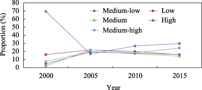
Fig. 2 Changes in the proportions of different types of cities

3.1.2 Characteristics of spatial changes

The trend of urban spatial agglomeration with a high PM2.5 concentration is very significant. The Moran index values of China’s urban PM2.5 concentrations in 2000 and 2005 were 0.316 and 0.351, respectively. They passed the test at the 1% level, indicating that there is a significant positive correlation with air quality in Chinese cities, but the scale of agglomeration is still relatively small. In 2010, the Moran index of the PM2.5 concentrations in Chinese cities increased to 0.725 and passed the test at the 1% level, indicating that there is a significant positive correlation with air quality in Chinese cities, and that there has been a phenomenon of large-scale agglomeration. The Moran index of the Chinese urban PM2.5 concentrations dropped to 0.663 in 2015, meaning that the agglomeration trend had weakened relative to the earlier period.
From the national perspective, city agglomeration with high PM2.5 concentrations changed from the individual region to multiple regions, and then to the large scale in contiguous areas (Fig. 3). In 2000, cities with high PM2.5 concentrations were mostly concentrated in the junction area of Shanxi, Shandong and Henan, while cities with medium-high PM2.5 concentrations were distributed around a small number of clusters. In 2005, the distribution range of cities with high PM2.5 concentrations was greatly expanded and formed four agglomerations with different scales of “one major and three minor concentrations” in the middle reaches of the Yangtze River and the Chengdu Plain. The cities with medium-high PM2.5 concentrations are mainly located in the areas between Beijing-Tianjin-Hebei and the Yangtze River Delta, and the periphery of core agglomeration areas of Wuhan and Chengdu. In 2010, the agglomeration scale of the cities with medium-high PM2.5 concentrations was adjusted, mainly in the North China Plain and the middle reaches of the Yangtze River with an expanding trend, while the Yangtze River Delta and Chengdu Plain agglomeration areas disappeared, and cities with medium-high PM2.5 concentrations were distributed around these agglomerations. In 2015, the distribution of cities with medium-high PM2.5 concentrations expanded again, and the North China agglomeration area and the Yangtze River agglomeration area became connected. At the same time, the Harbin-Changchun agglomeration zone emerged, and cities with medium-high PM2.5 concentrations were distributed around it.
Fig. 3 Temporal and spatial distributions of the PM2.5 concentrations in Chinese cities during 2000-2015
In addition, there are significant differences in PM2.5 concentrations among the major urban agglomerations, and they show expanding trends over time (Fig. 4). In 2000, the average concentration of PM2.5 in the Central Plains urban agglomeration was the highest, reaching 46.23 μg m-3; while the average concentration of PM2.5 in the Strait urban agglomeration was the lowest at only 21.34 μg m-3. Note that the former is 2.17 times the latter. In 2015, the average PM2.5 concentration of the Beijing-Tianjin-Hebei urban agglomeration was the highest, reaching 68.87 μg m-3; while the average PM2.5 concentration of the Strait urban agglomeration was still the lowest at only 27.62 μg m-3. The former is 2.49 times the latter. The changes in PM2.5 concentrations in urban agglomerations also show different trends over time. The Beijing-Tianjin-Hebei and Harbin-Changchun urban agglomerations show continuous upward trends, while the Yangtze River Delta and Central Plains urban agglomerations show increases. On the contrary, the Pearl River Delta and the west bank of the Taiwan Strait show the characteristics of rising at first and then falling.
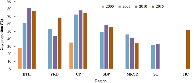
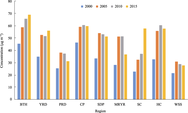
Fig. 4 The changes of PM2.5 concentrations in nine city agglomerations during 2000-2015

Note: BTH: Beijing-Tianjin-Hebei; YRD: Yangtze River Delta; PRD: Pearl River Delta; CP: Central Plains; SDP: Shandong Peninsula; MRYR: Middle Reaches of Yangtze River; SC: Sichuan-Chongqing; HC: Harbin-Changchun; WSS: The West Side of the Strait. The abbreviations of the regional names in other figures are the same as indicated here.

Figures 5 and 6 illustrate that the number and proportion of cities with high PM2.5 concentrations in each urban agglomeration show similar trends, but the changes in the internal structure of each urban agglomeration are different. In 2000, cities with high PM2.5 concentrations were concentrated in the Central Plains and Beijing-Tianjin-Hebei urban agglomerations. The numbers of cities with high PM2.5 concentrations were 35 and 28, respectively, accounting for 35% and 28% of the urban agglomeration cities. In 2015, the cities with high PM2.5 concentrations were mainly concentrated in the Central Plains, Yangtze River Delta, and Beijing-Tianjin-Hebei urban agglomerations. The numbers of cities with high PM2.5 concentrations were 101, 99, and 77, accounting for 74%, 68%, and 77% of the urban agglomeration cities, respectively. In general, the numbers of cities with high PM2.5 concentrations in the urban agglomerations of Chengdu, Chongqing, and the middle reaches of the Yangtze River each year and their proportions among all cities are relatively small. There are no cities with high PM2.5 concentrations in the two urban agglomerations of the Pearl River Delta and the west bank of the Strait.
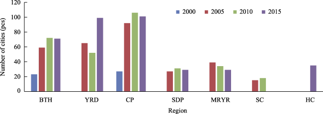
Fig. 5 The changes of the numbers of cities with high PM2.5 concentrations in each city agglomeration
Fig. 6 The changes of the proportions of cities with high PM2.5 concentrations in each city agglomeration

3.2 Factors influencing the PM2.5 concentration

In order to avoid the impacts of collinearity on the direction of model parameter estimation and the reliability of the statistical tests, correlation analysis and variance expansion factor were used to diagnose collinearity among the 12 selected indicators. The results show that there is no severe collinearity among these indicators. To alleviate the possible heteroscedasticity problem in the model, a logarithmic transformation was performed on the dependent and independent variables of the model before regression analysis in order to make the data more consistent with the normal distribution required by parameter estimation, thereby eliminating the heteroscedasticity of the model. On this basis, Stata15.0 software was used to estimate the parameters of the general linear model and the spatial measurement model (Table 2). After a comprehensive comparison, the spatial lag model was chosen. The estimation result of the spatial lag model is better than either the ordinary linear regression model or the spatial error model.
Table 2 The analysis of factors affecting the PM2.5 concentrations in Chinese cities by Ordinary Least Squares (OLS) and the Spatial Lag Model (SLM)
Variable 2000 2005 2010 2015
OLS SLM OLS SLM OLS SLM OLS SLM
ln EMMEAN -0.018 0.014 -0.046*** -0.028*** -0.070*** -0.040*** -0.102*** -0.048***
(0.014) (0.011) (0.009) (0.008) (0.010) (0.008) (0.012) (0.009)
ln DEMSTD -0.073*** -0.047*** -0.070*** -0.045*** -0.063*** -0.039*** -0.083*** -0.058***
(0.015) (0.011) (0.009) (0.008) (0.010) (0.008) (0.012) (0.009)
ln AVRAIN -0.348*** -0.074** -0.311*** -0.137*** -0.424*** -0.159*** -0.290*** -0.069***
(0.032) (0.031) (0.026) (0.023) (0.023) (0.023) (0.027) (0.023)
ln AVTEMP 0.301*** -0.011 0.231*** 0.049** 0.273*** 0.023 -0.112* -0.328***
(0.037) (0.035) (0.027) (0.024) (0.022) (0.022) (0.058) (0.029)
ln WIND -0.133** -0.279*** -0.464*** -0.599*** -0.512*** -0.540*** -0.665*** -0.497***
(0.056) (0.049) (0.050) (0.040) (0.052) (0.042) (0.092) (0.061)
ln NDVI 0.151 -0.200*** 0.104 -0.011 0.406*** 0.111** 0.103 0.093**
(0.093) (0.067) (0.077) (0.043) (0.068) (0.047) (0.072) (0.042)
ln PERGDP 0.029* -0.005 0.062*** 0.025*** 0.059*** 0.007 0.034** 0.002
(0.015) (0.013) (0.010) (0.008) (0.014) (0.012) (0.016) (0.013)
ln TNL 0.030* 0.042*** 0.016 0.018** 0.053*** 0.039*** 0.042*** 0.033***
(0.017) (0.013) (0.010) (0.008) (0.012) (0.010) (0.013) (0.008)
ln POPDES 0.131*** 0.078*** 0.159*** 0.098*** 0.120*** 0.077*** 0.101*** 0.067***
(0.021) (0.016) (0.014) (0.010) (0.017) (0.012) (0.015) (0.010)
ln ROAD -0.017 -0.002 0.020 0.028** 0.058*** 0.051*** -0.027** -0.015*
(0.022) (0.020) (0.014) (0.012) (0.016) (0.012) (0.013) (0.009)
ln COMPACT 0.112 0.315*** 0.091** 0.049 0.156*** 0.097** 0.014 -0.007
(0.073) (0.120) (0.045) (0.040) (0.049) (0.043) (0.052) (0.044)
ln CLUSDEGREE 0.024** -0.550** 0.037*** 0.037*** 0.031*** 0.034*** 0.046*** 0.028***
(0.011) (0.247) (0.008) (0.006) (0.008) (0.006) (0.007) (0.006)
Constant 3.106*** 2.403*** 4.594*** 4.569*** 5.037*** 4.535*** 7.470*** 5.906***
(0.258) (0.259) (0.223) (0.179) (0.226) (0.179) (0.406) (0.264)
ρ 0.308*** 0.207*** 0.210*** 0.226***
(0.016) (0.009) (0.010) (0.010)
Obs 751 751 1065 1065 1073 1073 1086 1086
R2 0.369 0.559 0.559 0.683 0.568 0.681 0.505 0.652
adjR2 0.358 0.554 0.563 0.499
F/Wald chi2 35.90 1024.16 111.99 2417.75 118.64 2448.91 99.61 2150.47

Note: Standard deviations are shown in brackets; ***, ** and * represent the significance levels of 1%, 5% and 10%, respectively.

Natural factors are the dominant factors affecting the urban PM2.5 concentration. From the perspective of topography, an average altitude above 1% in years other than 2000 has a significant negative impact on the urban PM2.5 concentration. This means that a higher average altitude is more conducive to the diffusion of the urban PM2.5. Compared with other natural factors, the average altitude has a smaller impact on the urban PM2.5 concentration, but this impact gradually increases over time. The degree of topographic undulation has a significant negative impact on the urban PM2.5 concentration in each year, and this impact remains stable on the whole.
From the perspective of meteorological conditions, wind speed, rainfall and temperature all affect the urban PM2.5 concentration significantly. Wind speed has the greatest impact on the urban PM2.5 concentration, followed by rainfall. Wind speed has a significant negative impact on the urban PM2.5 concentration in all years at the 1% significance level. It is worth noting that the magnitude of the impact shows the characteristics of first increasing and then decreasing, which may be related to the internal structures of the cities. Rainfall has a negative impact on the urban PM2.5 concentration in all years, which is significant at the 1% level. However, this impact has gradually weakened over time. The average annual temperature change has a stronger impact on the urban PM2.5 concentration, but this impact presents an inconsistent direction. Before 2010, it had a positive impact on the urban PM2.5 concentration, but in 2015 it had a negative impact. This change in direction may be due to the expansion of the cities and the increase in the heat island effect associated with it, which reduced the frequency of smog in the urban areas while the smog in the suburbs increased.
Except for the negative impact of the vegetation index on the urban PM2.5 concentration in 2000, this factor has a significant positive impact in other years. This conclusion is inconsistent with existing research, and this disparity may be related to the transformation of the urban PM2.5 distribution from a point-like distribution to a one-sided distribution after 2000. Although most cities have increased vegetation coverage, the vegetation conditions are no longer effective in reducing the urban PM2.5 concentrations.
Socio-economic factors are the key factors affecting the urban PM2.5 concentration. The per capita GDP has a positive impact on the urban PM2.5 concentration, which is consistent with expectations. This impact was significant for all years except 2015. At the same time, the per capita GDP has a relatively small impact on the urban PM2.5 concentration. As an important indicator of urban energy consumption, the total amount of city light usage at night has a considerable positive impact on the urban PM2.5 concentration in all years, and it is significant at the 5% level. Over time, the size of this impact has remained basically stable. Population density is an important indicator for measuring the social and economic intensity of the city. In all years, population density has a significant positive impact on the urban PM2.5 concentration. Furthermore, the impact of urban population density on the urban PM2.5 concentration presents a characteristic of first rising and then falling.
Urban morphology and structure are important factors affecting the urban PM2.5 concentration. The urban road network density has a significant impact on the urban PM2.5 concentration in all years except 2000. This impact had changed from positive before 2010 to negative in 2015, possibly due to the continuous increase in the urban road network density before 2010. However, the rate of urban car ownership increased, thus leading to severe traffic congestion in many cities. In recent years, some large cities have implemented traffic restriction systems within the cities while building rail transit and rapid transit to alleviate traffic emissions. The urban shape index has a significant positive impact on the urban PM2.5 concentration in most years, which indicates that the closer the urban planar shape is to a circle, the higher the urban PM2.5 concentration. However, this impact declines over time. The degree of urban agglomeration has a significant positive impact on the urban PM2.5 concentration in all years, but the impact is negative at first and then positive. The possible reason is that when the city is small, the high concentration of economic activities will help to reduce PM2.5 emissions, but with the expansion of the city scale and the increase of private cars, the urban population and socio-economic activities become highly concentrated in a few places within the city, and so the urban PM2.5 concentration also increases. Over time, the size of this impact remained basically stable.

4 Discussion

From the analysis of PM2.5 concentration changes in Chinese cities, the number of cities with high PM2.5 concentrations changed the most from 2000 to 2015, increasing from 16 cities in 2000 to 263 cities in 2015, for an increase of 247 cities in 15 years. The change in the number of cities with a moderately high PM2.5 concentration ranked second, from 521 in 2000 to 323 in 2015, for a decrease of 198 in 15 years, and the proportions of different types of cities show different characteristic stages. Among them, the cities with high PM2.5 concentrations showed an N-type fluctuation increase, while the cities with medium-high PM2.5 concentrations showed a V-type fluctuation increase. The area in which the high PM2.5 concentrations were the most concentrated has gradually expanded from the intersection area of Hebei, Shandong and Henan in the initial stage of the study to the whole North China Plain, the middle Yangtze River and the Harbin-Changchun region. This change is closely related to local economic development, natural factors, urban form and structure and other factors, and the natural factors are the stronger influencing factors.
The air pollution status of Chinese cities was discussed with respect to the changes in PM2.5 concentration, and the track of PM2.5 concentration changes in Chinese cities was clearly explained from the perspectives of time and space. From 2000 to 2015, China was in the stage of rapid economic and social development, and urban economic development made remarkable achievements. The study of PM2.5 concentrations in Chinese cities can provide warnings for the healthy development of cities, paying attention to the coordinated relationship between economic development and environmental construction and pursuing the coordinated development of the two, in order to achieve the high-quality economic and social development of Chinese cities.
Urban night lights are used to represent urban energy consumption. Although this factor is representative to a certain extent, there are also objective errors, so there is room for further optimization in the measurement results of urban PM2.5 concentrations. At the same time, although this study chose 2000-2015 as the research stage, when China's economy developed rapidly, there is still a large time gap between 2015 and the present. Due to data limitations, it is impossible to effectively track the latest situation of PM2.5 concentration changes in Chinese cities. Therefore, although this study demonstrates the spatial-temporal development of PM2.5 concentrations in Chinese cities, it has limited practical guidance significance. As a result, it is necessary to carry out additional research on topics such as urban low-carbon and healthy development based on the background of China’s carbon peak and carbon neutrality strategy.

5 Conclusions and policy implications

This paper dynamically identifies the scope of urban built-up areas based on the combination of urban construction land and population density. On this basis, exploratory spatial analysis and spatial econometric analysis methods were used to analyze the temporal and spatial evolutionary characteristics and factors influencing the annual average PM2.5 concentration in Chinese cities. This analysis led to four main conclusions.
First, China’s overall urban PM2.5 concentration showed an inverted L-shaped increase from 2000 to 2015, namely a sharp increase before 2005 and slow growth after 2005. Cities with high PM2.5 concentrations show the largest changes, followed by low PM2.5 concentrations; while cities with low PM2.5 concentrations have the largest changes and their PM2.5 concentrations are high. However, the changes in the numbers and proportions of different types of cities present differential phase characteristics. In particular, cities with high PM2.5 concentrations show an increase in N-shaped fluctuations, while cities with medium-low PM2.5 concentrations show an increase in inverted V-shaped fluctuations.
Second, from the perspective of spatial distribution, the trend of spatial agglomeration in cities with high PM2.5 concentrations is significant. In 2000, small-scale agglomeration was seen in the junction area of Hebei, Shandong and Henan; in 2005, the scope of agglomeration expanded to Beijing-Tianjin-Hebei, the middle Yangtze River, the Yangtze River Delta and the Chengdu Plain; in 2015, it grew to cover the entire North China Plain, the middle Yangtze River, and the Harbin-Changchun region. The urban agglomeration north of the Yangtze River has a high PM2.5 concentration. The numbers and proportions of cities with high PM2.5 concentrations in the Central Plains and Beijing-Tianjin-Hebei urban agglomerations were relatively high. At the same time, there were no cities with high PM2.5 concentrations in the Pearl River Delta or the west bank of the Straits. The changes in PM2.5 concentrations and the structures of various urban agglomerations show different trends.
Third, the concentrations of PM2.5 in Chinese cities are affected by natural factors, socio-economic factors, and urban morphological and structural factors. The elastic coefficient of natural factors is greater than those of social-economic factors and urban morphological and structural factors. Generally, average wind speed exerts the most significant impact among the natural factors, successively followed by average rainfall, average temperature, vegetation coverage, terrain undulation and altitude. Among socio-economic factors, population density exerts the most significant impact, successively followed by energy consumption and per capita GDP. Among urban morphology factors, urban population agglomeration degree exerts the most significant impact, successively followed by road network density and compact degree. Over time, the sizes and directions of the effects of the various indicators will change.
Based on the above findings, this study provides the following policy implications. The urban PM2.5 concentration is affected by natural factors, socio-economic factors, urban form and structure. The results show that the elastic coefficient of natural factors to urban PM2.5 concentration is generally greater than those of socioeconomic factors and urban morphology and structure factors. This conclusion is in line with research on the Beijing-Tianjin-Hebei region (Wu et al., 2014). However, it is difficult to make significant changes in natural factors such as topographic undulation, annual average temperature, and average annual rainfall. These factors can be regarded as “inelastic”. At the same time, natural factors do not produce pollution and only affect the spread of urban PM2.5 pollution. Although socio-economic factors and urban morphology and structure have a relatively small impact on the elasticity coefficient, appropriate policies and measures can be adopted to change it. We can pursue targeted strategies to prevent and control urban PM2.5 pollution, such as establishing a cross-administrative coordination mechanism consisting of the transformation of development modes, energy structure transformation, and comprehensive pollution prevention, developing multi-center cities, building urban air ducts, increasing the land use mix, and optimizing urban morphology and structure.
The major limitation of this study is that it cannot incorporate the existing statistical yearbook data, so some factors that may affect the urban PM2.5 concentration, such as car ownership, economic structure, and separation of occupation and residence, cannot be included in the models. At the same time, with the accumulation of urban big data such as mobile phone signaling data and car navigation data, future research can incorporate more potential influencing factors into the analysis.
[1]
Beckett K P, Freer-Smith P H, Taylor G. 2000. Particulate pollution capture by urban trees: Effect of species and windspeed. Global Change Biology, 6(8): 995-1003.

[2]
Boone C G, Fragkias M, Buckley G L, et al. 2014. A long view of polluting industry and environmental justice in Baltimore. Cities, 36: 41-49.

[3]
Center for International Earth Science Information Network. 2004. Global Rural-Urban Mapping Project (GRUMP), alpha version:Urban extents. New York, USA: Center for International Earth Science Information Network (CIESIN), University of Chicago.

[4]
Ewing R, Cervero R. 2010. Travel and the built environment. Journal of the American Planning Association, 76(3): 265-294.

[5]
Hankey S, Marshall J D. 2010. Impacts of urban form on future US passenger-vehicle greenhouse gas emissions. Energy Policy, 38(9): 4880- 4887.

[6]
Lee C. 2020. Impacts of multi-scale urban form on PM2.5 concentrations using continuous surface estimates with high-resolution in US metropolitan areas. Landscape and Urban Planning, 204: 103935. DOI: 10.1016/j.landurbplan.2020.103935.

[7]
Li J M, Han X L, Jin M J, et al. 2019. Globally analysing spatiotemporal trends of anthropogenic PM2.5 concentration and population’s PM2.5 exposure from 1998 to 2016. Environment International, 128: 46-62.

[8]
Li W M, Gao S J, Xu J. 2018. The green growth progress and countermeasure of China in the view of international comparison. Reform, (12): 27-41. (in Chinese)

[9]
Lin D, Allan A, Cui J Q. 2015. The impacts of urban spatial structure and socio-economic factors on patterns of commuting: A review. International Journal of Urban Sciences, 19(2): 238-255.

[10]
Liu H, Fang C, Huang J, et al. 2018. The spatial-temporal characteristics and influencing factors of air pollution in Beijing-Tianjin-Hebei Urban Agglomeration. Acta Geographica Sinica, 73(1): 177-191. (in Chinese)

[11]
Ma X, Wang C Y, Han G, et al. 2019. Regional atmospheric aerosol pollution detection based on LiDAR remote sensing. Remote Sensing, 11(20): 23-39.

[12]
Maharjan S, Tsurusaki N, Divigalpitiya P. 2018. Influencing mechanism analysis of urban form on travel energy consumption—Evidence from Fukuoka City, Japan. Urban Science, 2(1): 15. DOI: 10.3390/urbansci2010015.

[13]
Marcińczak S, Bartosiewicz B. 2018. Commuting patterns and urban form: Evidence from Poland. Journal of Transport Geography, 70: 31-39.

[14]
McCarty J, Kaza N. 2015. Urban form and air quality in the United States. Landscape and Urban Planning, 139: 168-179.

[15]
Stead D. 2001. Relationships between land use, socioeconomic factors, and travel patterns in Britain. Environment and Planning B: Planning and Design, 28(4): 499-528.

[16]
Su Q. 2011. The effect of population density, road network density, and congestion on household gasoline consumption in US urban areas. Energy Economics, 33(3): 445-452.

[17]
Wang S J, Liu X P, Yang X, et al. 2018. Spatial variations of PM2.5 in Chinese cities for the joint impacts of human activities and natural conditions: A global and local regression perspective. Journal of Cleaner Production, 203: 143-152.

[18]
Wu J S, Niu Y, Peng J, et al. 2014. Research on energy consumption dynamic among prefecture-level cities in China based on DMSP/OLS Nighttime Light. Geographical Research, 33(4): 625-634. (in Chinese)

[19]
Yan L X, Duarte F, Wang D, et al. 2019. Exploring the effect of air pollution on social activity in China using geotagged social media check-in data. Cities, 91: 116-125.

[20]
Yang Y, Li X R, Shen R R, et al. 2020. Seasonal variation and sources of derivatized phenols in atmospheric fine particulate matter in North China Plain. Journal of Environmental Sciences, 89: 136-144.

[21]
Yuan M, Song Y, Huang Y P, et al. 2019. Exploring the association between the built environment and remotely sensed PM2.5 concentrations in urban areas. Journal of Cleaner Production, 220: 1014-1023.

[22]
Zhang N N, Ma F, Qin C B, et al. 2018. Spatiotemporal trends in PM2.5 levels from 2013 to 2017 and regional demarcations for joint prevention and control of atmospheric pollution in China. Chemosphere, 210: 1176-1184.

Outlines

/