Resource Economy

The Impact of the Spatial Agglomeration of Producer Services on Urban Productivity

  • ZHOU You , 1, 2, *
Expand
  • 1. School of Economics, Hunan University of Finance and Economics, Changsha 410205, China
  • 2. Post-Doctoral Station of Chinese History, Hunan Normal University, Changsha 410081, China
*ZHOU You, E-mail:

Received date: 2022-01-07

  Accepted date: 2022-05-20

  Online published: 2023-02-21

Supported by

The National Natural Science Foundation of China(71903050)

The Key project of Hunan provincial Social Science Achievement Review Committee(XSP2023ZDI014)

China Postdoctoral Science Foundation(2021T140199)

The General Project of Hunan Natural Science Foundation(2021jj30072)

The Excellent Youth Project of Hunan Provincial Department of Education(21B0840)

The 65th Batch of General Funded Projects of China Postdoctoral Science Foundation(2019M652779)

Abstract

The spatial cluster effect of productive service industry agglomeration and the urban productivity level in 286 prefecture level cities in China during 2008-2018 were analyzed by using the Moran index and the Lisa cluster diagram. The results show that the spatial correlation between productive service industry agglomeration and urban productivity is high, as the high-value areas of producer services agglomeration are generally the high-value agglomeration areas of China’s urban productivity level, while the low-value areas of producer services agglomeration are generally the low-value agglomeration areas of China’s urban productivity level. Furthermore, the spatial econometric model was used to test the effect of producer services agglomeration on urban productivity in China. The results show that producer services agglomeration can effectively improve urban productivity in China, but its impact on the productivity in different cities is quite variable. The producer services specialization agglomeration on urban productivity in eastern China is more obvious, while the positive effect of the diversification agglomeration of producer services on urban productivity is more obvious in the West, the Central and the Northeast, but the promotion of eastern cities is less apparent.

Cite this article

ZHOU You . The Impact of the Spatial Agglomeration of Producer Services on Urban Productivity[J]. Journal of Resources and Ecology, 2023 , 14(2) : 344 -356 . DOI: 10.5814/j.issn.1674-764x.2023.02.012

1 Introduction

At present, China is vigorously implementing the new urbanization development strategy. Urbanization is not only an important starting point for realizing China’s industrialization and modernization, but it also has the potential to promote China’s domestic demand growth and to serve as the driving force of economic development. In 2020, China’s urbanization rate will reach 63.89%, and the urban economy will become the key engine of China’s economic growth and sustainable development. However, after the miracle of rapid economic growth, achieving high-quality economic development has become an urgent problem to be solved. The development of the urban economy and the improvement of urban productivity are the keys to the high-quality and intensive development of China’s economy. They are also the fundamental requirements for promoting the transformation and upgrading of urbanization in the new stage of economic development. According to the National Bureau of statistics data, in 2020, the total output value of China’s service industry accounted for 54.5% of the GDP and contributed 60% to GDP growth. Compared with the secondary industry, the service industry has a stronger agglomeration economy and technology spillover effect, and the producer service industry with the characteristics of high technology and high employment is the development direction of the service industry in the future. In view of this, the 14th five year plan for national economic and social development and the long-term goal for 2035 clearly emphasize the need to promote the extension of producer services to more specialized and high-end levels, and to promote the agglomeration of producer services in central cities, so as to optimize urban industrial institutions and improve urban productivity. The 14th Five-Year Plan report also pointed out that we should guide the modern service industry to cluster in central cities and boost the transformation and upgrading of the manufacturing industry. Promoting the agglomeration of producer services in cities is an important breakthrough for deepening the division of labor, guiding the population and industrial agglomeration, and then effectively promoting urban productivity.
Producer services agglomeration is not only conducive to the formation of a labor division network among producer service enterprises, but it also promotes the industrial linkage between producer service enterprises and manufacturing enterprises, realizes the effect of economies of scale, and ultimately promotes the improvement of urban productivity. As for the mechanism of producer services agglomeration on urban productivity, Marshall (1961) and Jacobs (1969) provided a basic explanation. Marshall believed that the agglomeration of manufacturers in the same industry is conducive to the sharing of knowledge and technology among enterprises, and the technical externality comes from the specialized division of labor of the enterprises. Jacobs, from the perspective of diversified agglomeration of producer services, believed that the agglomeration of manufacturers in different industries will produce a gradual increase in scale and income. Both specialized agglomeration and diversified agglomeration will produce technological externality, which is an important source for improving urban productivity and optimizing the urban industrial structure (Glaeser et al., 1992). The agglomeration of producer services is conducive to the agglomeration of highly skilled talents and the technological connection between upstream and downstream enterprises, and to the generation and exchange of new knowledge. It mainly promotes the improvement of urban productivity by promoting technological progress (Li, 2019; Chen and Zhou, 2020). The above research shows that producer services agglomeration will drive the urban economy to obtain technological effects, but it has not identified which model this technology effect comes from. Other scholars found through research that producer services agglomeration did not significantly improve urban productivity. For example, Andersson (2006) found that although producer services agglomeration promoted the improvement of manufacturing efficiency, the effect was not significant. Similarly, Xu (2010) found that the service industry does not have its own characteristics of enhancement, and the improvement effect on industrial efficiency is not obvious. Lv and Ren (2017) conducted an empirical analysis based on the panel data model of 41 cities from 2003 to 2014. Their results showed that the development of producer services has a certain threshold effect on the promotion of urban productivity, and the development of producer services in some cities in the Yangtze River Delta had not yet reached the stage of improving productivity. In similar studies, Liu and Song (2007) found that the economic effect of producer services is lower than that of manufacturing, mainly due to the higher amount of equipment assets required per unit labor in producer services. In recent studies, some scholars have turned their research focus to the perspective of spatial correlations between producer services agglomeration and urban productivity improvement, such as Chen’s (2021) investigation on the impact of producer services agglomeration on urban productivity in 261 cities in China, and Zhang et al. (2019) who tested the impact of producer services agglomeration and its spatial spillover effect on green total factor productivity in 30 provinces and cities in China. In addition, relevant studies have shown that the market scale, traffic conditions, foreign direct investment, investment in scientific and technological innovation, human capital and other factors in different regions also have profound impacts on urban productivity. Therefore, there may be regional differences in the spillover effect of producer service agglomeration on urban productivity.
Due to the differences in research methods and index selection, the existing research on the specific effects of producer services agglomeration on urban productivity has not produced consistent results. It is one-sided in that only the effect of the same industrial specialization agglomeration or different industrial diversification agglomerations on urban productivity have been studied. In addition, most of the existing studies examine the producer service industry agglomeration at the industrial level based on time series or panel data, and there is little in-depth research from the perspective of spatial correlation. When the impact of the spatial correlation of variables on the model is not considered, the empirical results may be biased. In view of this limitation, this study analyzes the spatial correlations between the professional agglomeration and diversified agglomeration of producer services and urban productivity by combining the technology externality theory of Marshall and Jacobs, and further constructs a spatial econometric model to comprehensively investigate the overall level and sub-sectors of the impact of producer services agglomeration on urban productivity.

2 Exploratory spatial data analysis of producer service agglomeration and urban productivity

The Moran index and scatter diagram are first used to analyze the cluster effect of producer services and urban productivity in geographical space, and then the local spatial correlation index Lisa cluster diagram is further used to test the spatial correlation between producer services agglomeration and urban productivity. The sample objects are the data of 286 cities in China from 2008 to 2018. The data were obtained from the China Urban Statistical Yearbook, China Urban Construction Statistical Yearbook and CEIC China economic database for these years.

2.1 Spatial autocorrelation test

The Moran index can detect the spatial correlations of variables, and its value range is [-1, 1]. When the Moran index value is greater than zero and closer to 1, it indicates that the spatial positive dependence of the variables is stronger. On the contrary, it indicates that there is a spatial negative correlation.
The Moran value of producer services agglomeration. According to the sub-industry statistical caliber of service industry employment in China’s urban statistical yearbook, nine industries with productive characteristics are classified(① These nine industries are electricity and gas water supply, construction, transportation, warehousing and postal services, information transmission, computer services and software, wholesale and retail, finance, leasing and commercial services, scientific and technological services and geological exploration, water conservancy environment and public facilities management.), and identified as the producer services (Zhou and Tan, 2016). The specialized agglomeration (MI) of producer services draws on the calculation method of Ezcurra (2006), and the specific indicators are as follows:
${{M}_{i}}=\underset{j}{\mathop{\mathop{\sum }^{}}}\,\left| \frac{{{E}_{ij}}}{{{E}_{i}}}-\frac{{{{{E}'}}_{j}}}{{{E}'}} \right|$
where Eij/Ei represents the ratio of the number of employed persons in j industry in i city to the total number of employed persons in the city, and E'j/E' represents the ratio of the number of employed persons in j industry in the country (except for i city) to the total number of employed persons in the country (except for i city). This index is used to characterize the “Marshall technology externality”.
In order to take the economic weights of various industries and the comparability of industries at different levels into account, the improved Hefendal Hirschman index (Combes, 2000) is used to measure the diversified agglomeration of producer services. The specific equation is as follows:
${{D}_{i}}=\underset{j}{\mathop{\mathop{\sum }^{}}}\,\frac{{{E}_{ij}}}{{{E}_{i}}}\times \left[ \frac{\underset{{j}'=1,{j}'\ne j}{\overset{n}{\mathop{\mathop{\sum }^{}}}}\,{{\left( \frac{{{E}_{{{j}'}}}}{E-{{E}_{j}}} \right)}^{2}}}{\underset{{j}'=1,{j}'\ne j}{\overset{n}{\mathop{\mathop{\sum }^{}}}}\,{{\left( \frac{{{E}_{i{j}'}}}{{{E}_{i}}-{{E}_{ij}}} \right)}^{2}}} \right]$
In equation (2), Eij, Ei and E'j are the same as in equation (1), while Ej and E respectively represent the employment of j industry and the total employment of the country, and Eij' represents the employment of j' in a productive service industry other than industry j in i city. This index value is used to characterize the “Jacobs technology externality”.
The Moran values of producer service specialization agglomeration and diversification agglomeration are shown in Table 1. It is easy to see that the Moran values of the producer service specialization and diversification agglomeration variables are positive and significant at the 10% significance level, indicating that the spatial distribution of producer service agglomeration is not random, but shows a positive correlative phenomenon.
Table 1 Moran index values of producer services agglomeration and urban productivity from 2008 to 2018
Year Professional agglomeration of
producer services (SP)
Diversified agglomeration of
producer services (DV)
Urban productivity (CP)
Moran Value of Z Value of P Moran Value of Z Value of P Moran Value of Z Value of P
2008 0.2397 2.7339 0.0280 0.3011 7.2405 0.0000 0.3934 8.9295 0.0000
2009 0.2786 3.1120 0.0060 0.3003 6.9101 0.0000 0.3875 8.1123 0.0000
2010 0.2817 3.2152 0.0059 0.2951 6.8716 0.0000 0.3648 8.3356 0.0000
2011 0.2919 3.3315 0.0028 0.3021 7.0123 0.0000 0.4064 8.1159 0.0000
2012 0.3012 3.6452 0.0021 0.3617 7.9803 0.0000 0.3983 5.0906 0.0892
2013 0.2498 2.8877 0.0168 0.2740 5.6689 0.0000 0.3896 7.9953 0.0000
2014 0.2325 2.4723 0.0310 0.2509 5.1562 0.0000 0.3778 7.8650 0.0000
2015 0.2401 2.7661 0.0179 0.2778 6.1101 0.0000 0.0988 8.1167 0.0000
2016 0.2652 3.0010 0.0067 0.2910 6.2391 0.0000 0.3994 7.6875 0.0000
2017 0.2633 2.9716 0.0071 0.3061 6.3744 0.0000 0.3769 7.3892 0.0000
2018 0.2382 2.5413 0.0307 0.2879 6.2305 0.0000 0.3790 8.0503 0.0000
Referring to the practices of Zhang and Zhang (2017), the indicator of urban labor productivity adopts the labor productivity of non-agricultural industries, that is, the total value of urban per capita secondary and tertiary industries. The data in Table 1 show that the Moran value of urban productivity passed the test at the 5% significance level in all years except for 2010, and the Moran value in 2013 was the lowest at 0.0988. Therefore, there is also a cluster phenomenon in the spatial distribution of the urban productivity level in China.
The coordinates in the Moran index scatter chart define four quadrants, which respectively represent different cluster modes. The first quadrant represents high-high agglomeration (that is, cities with high agglomeration levels are surrounded by other cities with high agglomeration levels), the second quadrant represents low-high agglomeration (that is, cities with low agglomeration levels are surrounded by other cities with high agglomeration levels), and the third and fourth quadrants represent low-low agglomeration and high-low agglomeration modes, respectively. Based on the Moran scatter diagram distribution of producer services and urban productivity, most cities are located in the first and third quadrants, indicating that cities with producer services agglomeration and high urban productivity are surrounded by other cities with the same high level, while cities with low levels are also concentrated in space.

2.2 Spatial correlation local index based on the Lisa cluster diagram

Spatial autocorrelation analysis cannot reflect the spatial correlation mode of specific cities, while the Lisa cluster map can clearly describe the agglomeration modes of specific cities. The local Lisa cluster diagram of producer services agglomeration and urban productivity levels in 2008 shows that most cities’ professional agglomeration and diversified agglomeration of producer services were located in medium and low agglomeration areas (i.e., low-high (LH), high-low (HL) or low-low (LL) agglomeration modes), while cities along the coastline in the East were located in high-value agglomeration areas (i.e., high-high (HH) agglomeration mode). On the whole, in 2008, the spatial distribution of specialization and diversified agglomeration of urban producer services in China was not obvious. By 2018, driven by the coastal cities, the specialization and diversified agglomeration levels of producer services in mainland cities had become significantly improved. More and more cities are located in high-high agglomeration areas in 2018, basically forming a high-value agglomeration belt connected by coastal cities and a medium high-value agglomeration area connected by cities along the Beijing-Harbin and Beijing-Guangzhou Railway (mainly high-high and high-low agglomeration areas). Overall, the average agglomeration level of urban producer services increased significantly in 2018. The advantages of producer services agglomeration in eastern cities have driven the improvement of producer services agglomeration levels in other cities to a certain extent.
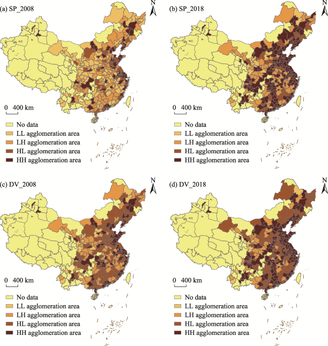
Fig. 1 Lisa cluster diagrams of producer services specialization agglomeration (SP) and diversification agglomeration (DV) in 2008 and 2018
The Lisa statistical chart of the urban productivity level (Fig. 2) shows that most of China’s urban productivity levels in 2008 were located at low and medium agglomeration levels (mainly low-high and low-low agglomeration areas). Although a small number of coastal cities were located in high-value agglomeration areas (high-high agglomeration), they did not form obvious agglomeration blocks. Generally speaking, the spatial distribution level of urban productivity in China in 2008 is not obvious. By 2018, the productivity levels of cities in all sectors were significantly improved, forming high-value agglomeration areas composed of urban agglomerations in the Yangtze River Delta, Pearl River Delta and Bohai Rim, medium- and high-value agglomeration areas composed of central cities such as Hunan, Hubei, Anhui and Henan (mainly high-high and high-low agglomeration) and low- and medium-value agglomeration areas composed of cities in western provinces such as Inner Mongolia, Shaanxi and Gansu (mainly low-low and low-high agglomeration). Generally speaking, the high-high agglomeration area of urban productivity included more and more cities in 2018, showing a trend that the coast drives the mainland and the center radiates into the surrounding areas.
From the perspective of the spatial cluster distribution of producer services agglomeration and urban productivity, there is a significant spatial correlation and obvious synchronization between them. The high-value areas of producer services agglomeration are generally the high-value agglomeration areas of China’s urban productivity level, while the low-value areas of producer services agglomeration are generally the low-value agglomeration areas of China’s urban productivity level. This also reflects the further development of the economy, so it is necessary to establish a spatial econometric model for empirical testing.
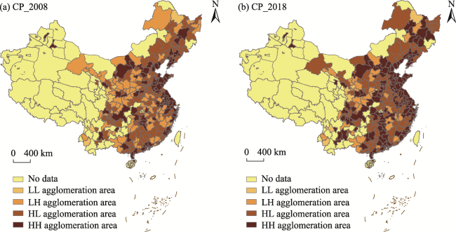
Fig. 2 Lisa cluster of urban productivity in 2008 and 2018

3 Empirical strategy and data description

3.1 Model setting

Based on the Cobb Douglas production function model, the function of producer service agglomeration affecting urban productivity is constructed. The basic production function of city i can be expressed as:
${{Y}_{it}}=AK_{it}^{\alpha }L_{it}^{\beta }$
In equation (3), Yit represents the output of city i in year t, K and L represent the capital factor and labor factor inputs, respectively, A represents technological progress; α and β respectively represents the output elasticity of capital and labor. Since the total urban output is mainly composed of the output of industry and the service industry, the per capita total urban output Y/L can be used to approximate the productivity (CP) of city i. By averaging equation (3), we get:
$C{{P}_{it}}=A({{Z}_{it}})K_{it}^{\alpha }L_{it}^{\beta -1}$
where CPit means urban productivity, A(Zit) is a Hicks multiplier and Zit is a factor affecting technological progress. Sub tables K and L represent the input of capital and labor factors per capita. According to the Marshall and Jacobs’ theory of technological externality, producer services agglomeration generally produces technological externality through specialization agglomeration (SP) and diversification agglomeration (DV). Therefore, the Hicks multiplier can be expressed as$A=f({{z}_{it}})={{A}_{0}}SP_{it}^{{{\delta }_{1}}}DV_{it}^{{{\delta }_{2}}}e$(e is the residual term), brought into equation (4) and taken as the logarithm which yields:
$\text{ln}C{{P}_{it}}={{T}_{0}}+{{\delta }_{1}}\text{ln}S{{P}_{it}}+{{\delta }_{2}}\text{ln}D{{V}_{it}}+\alpha \text{ln}{{k}_{it}}+\lambda \text{ln}{{L}_{it}}+{{\varepsilon }_{it}}$
where T0=lnA0, λ=β-1, εit=lneit, δ1 and δ2 represent the coefficients of producer service specialization agglomeration (SP) and producer service diversification agglomeration (DV) variables, respectively. In addition, in order to ensure the stability and accuracy of the regression results, market scale, traffic conditions, investment in scientific and technological innovation, foreign direct investment, human capital and other control variables commonly used in existing relevant studies were added to the model.
The previous analysis shows an obvious spatial autocorrelation in the level of urban productivity, and the specialization and diversified agglomeration of producer services enhance the spatial dependence of urban productivity. Therefore, spatial factors should be considered when analyzing the effect of producer services agglomeration on urban productivity. Anselin et al. (2008) proposed a spatial lag model (SLM) and a spatial error model (SCM) according to the impact mode difference of spatial correlation. The main difference between them is that the spatial lag model uses the coefficient of a spatial lag dependent variable to reflect the spatial dependence, while the spatial error model reflects the size of the spatial dependence in the error term of the model. Subsequently, James and Kelly (2009) extended the spatial lag model and incorporated the lag term of the explained variable and the explanatory variable into the model to obtain the spatial Dobbin model (SDM). Elhorst (2010) pointed out that the LM test can better judge which model to use. If there are both spatial error and spatial lag, and the test results reject the OLS model, then the spatial Dobbin model is more suitable. In this study, the LM test results show that the model passes the test at the 5% significance level, which shows that there is spatial autocorrelation between urban productivity and the influencing factors. In addition, the LM test results also reject the original assumption that there is no spatial correlation between urban productivity and the error terms. Therefore, it is more reasonable to use the spatial Dobbin model, and its basic form is:
$Y={{\lambda }_{1}}+{{\lambda }_{2}}X+\rho WY+\theta WX+\mu $
where Y is the dependent variable and X is the set of independent variables, ρWY and θWX represent the spatial lag terms of Y and X, respectively, and W represents the spatial weight matrix. In order to avoid the inaccuracy of the model results caused by neglecting the long-distance spatial relationship in the binary adjacency matrix, the following comprehensive geographic matrix measurement is constructed based on the findings of Hou et al. (2014):
${{W}_{ij}}=\left\{ \begin{matrix} Q/d_{ij}^{2},\ i\ne j \\ 0,\ \begin{matrix} {} & {} \\ \end{matrix}i=j \\ \end{matrix} \right.$
where Q represents the product of the average per capita GDP of cities i and j during 2008-2018, and dij is the distance between the centers of cities i and j.(② The data came from the survey and geographic network of the satellite positioning system Google Earth (www.geobytes.com/citydistance).)
Equation (5) is extended and the SDM model is adopted, and the resulting expression becomes:
$\begin{align} & \text{ln}C{{P}_{it}}=\rho \underset{j=1}{\overset{n}{\mathop{\mathop{\sum }^{}}}}\,{{W}_{ij}}\text{ln}C{{P}_{jt}}+{{T}_{0}}+{{\delta }_{1}}\text{ln}S{{P}_{it}}+{{\delta }_{2}}\text{ln}D{{V}_{it}}+ \\ & \ \ \ \ \ \ \ \ \ \ \ \alpha \text{ln}{{k}_{it}}+\beta \text{ln}{{L}_{it}}+\chi \text{ln}Co{{n}_{it}}+{{\eta }_{1}}\underset{j=1}{\overset{n}{\mathop{\mathop{\sum }^{}}}}\,{{W}_{ij}}\text{ln}S{{P}_{it}}+ \\ & \ \ \ \ \ \ \ \ \ \ \ {{\eta }_{2}}\underset{j=1}{\overset{n}{\mathop{\mathop{\sum }^{}}}}\,{{W}_{ij}}\text{ln}D{{V}_{it}}+{{\eta }_{3}}\underset{j=1}{\overset{n}{\mathop{\mathop{\sum }^{}}}}\,{{W}_{ij}}\text{ln}{{k}_{it}}+{{\eta }_{4}}\underset{j=1}{\overset{n}{\mathop{\mathop{\sum }^{}}}}\,{{W}_{ij}}\text{ln}{{L}_{it}}+ \\ & \ \ \ \ \ \ \ \ \ \ \ {{\eta }_{5}}\underset{j=1}{\overset{n}{\mathop{\mathop{\sum }^{}}}}\,{{W}_{ij}}\text{ln}Co{{n}_{it}}+{{d}_{i}}+{{v}_{t}}+{{\varepsilon }_{it}} \\ \end{align}$
where, η1, η2, η3, η4, η5 represent the coefficients of each variable after placing into the spatial weight matrix,Conit is the set of control variables, di and vt represent regional and time effects, and other variables and symbols are defined as above.

3.2 Index selection and data description

Due to the changes in some administrative divisions, such as Sansha and Bijie, and the serious lack of data in cities such as Lhasa, the sample data covers 286 other Chinese cities at the prefecture level and above from 2008 to 2018. The original data came from the urban statistical yearbook, provincial statistical yearbook, China Urban Construction Statistical Yearbook and CEIC China economic database for these years. The explanatory variables (urban productivity (CP)) and key explanatory variables (producer services specialization agglomeration (SP) and diversification agglomeration (DV)) in the model are described above. The per capita capital input is approximated by the stock of per capita fixed asset investment, which is calculated using the sustainable inventory method based on the calculation method of Zhang et al. (2004), and the labor input is measured by the number of employees in the municipal area.
The measurements of other control variables are as follows. 1) Market scale is expressed by regional consumption expenditure, which is used to reflect the impact of urban consumption level on labor productivity. 2) Investment in scientific and technological innovation is expressed by the per capita local financial budget of the municipal district, and it is used to reflect the innovation driving effect in the process of improving urban production efficiency. 3) Foreign direct investment (FDI): FDI not only increases the city’s capital stock, but also affects the city’s productivity through the technology spillover effect. It is measured by the stock of FDI actually used per capita, and the results are calculated by the sustainable inventory method. 4) Human capital (HC): The level of human capital not only affects the innovation ability of cities, but also relates to the management efficiency of enterprises. A high level of human capital is conducive to improving urban productivity. It is expressed here by the proportion of ordinary middle school and college graduates in the total local population. 5) Traffic conditions (TC) represent another important indicator affecting the efficiency of the urban economic agglomeration level, which is approximated by the per capita urban road area (m2). Table 2 shows the statistical values of sample data for these variables among the 286 urban cities in China.
Table 2 Statistical values of sample data for the variables of 286 urban cities in China for 2008-2018
Variable Mean Standard deviation Minimum Maximum Number of samples
CP (Urban productivity) 0.3472 0.2512 0.0356 0.8911 3146
SP (Professional agglomeration of producer services) 0.4811 0.2113 0.1210 1.7932 3146
DV (Diversified agglomeration of producer services) 0.9112 0.2210 0.3733 1.9024 3146
K (Per capita capital investment, ×104 yuan) 2.5732 7.4047 0.6333 11.0007 3146
L (Labor input, ×104 people) 103.5178 1812.4915 9.7900 2115.7700 3146
MS (Market scale, yuan) 8.9940 0.6581 6.8223 11.6972 3146
TRI (Investment in scientific and technological innovation, yuan) 3.6400 11341.6000 0.0643 201.5000 3146
FDI (Foreign direct investment, yuan) 800.2943 43221.3100 100.1142 3000.2855 3146
HC (Human capital) 0.1142 0.1281 0.0120 0.3341 3146
TC (Traffic conditions, m2) 7.1156 4.6531 0.6122 62.4785 3146

4 Measurement results and robustness test

4.1 Population sample estimation results

Before regressing the spatial Doberman model, it is necessary to determine whether to use the fixed effect model or the random effect model. The results of the Hausman test show that the alternative hypothesis is valid and the fixed effect model is more reasonable. According to the control of the fixed effect on space and time, it can be divided into a non-fixed effect, a space fixed effect, a time fixed effect and a fixed effect with space and time at the same time. The LR test is further used to judge whether there is a time effect and a regional effect. The results show that the impact effect of the structural difference between regions is significant, but the impact effect of the time difference is not significant. Therefore, the regional effect should be considered in the regression. The possible reasons include the fact that there are obvious spatial characteristics of productivity among the cities in China, and the changes in urban productivity mainly come from the differences between individuals in the cross section. Furthermore, the productivity of a city is not only impacted by the productivity of neighboring cities, but also by the error of regional structural differences, which are reflected in the agglomeration level of producer services, per capita capital and labor investment, market scale, investment in scientific and technological innovation, and foreign direct investment. There are also differences between spatial influencing factors such as human capital and traffic conditions. Therefore, the regression results in Table 3 show two sets of results: spatial Doberman no fixed effect and spatial Doberman fixed effect. It is clear that the estimation results of the spatial fixed effect model are better than those of the non-fixed effect model, whether measured by the goodness of fit index or the log likelihood value index, which shows that the stability and accuracy of the regression results are higher after considering the impact of inter-regional interactions. It also shows that there is a phenomenon of geographical agglomeration of urban productivity in China. The change in the urban productivity is mainly impacted by the productivity differences between cities in the same period. The productivity level of a city is not only impacted by the productivity level of neighboring cities, but it is also impacted by the error of structural differences between cities.
Regarding the spatial lag term of urban productivity, its regression coefficient ρ is significantly positive under the comprehensive geographical matrix, indicating that China's urban productivity has a strong positive correlation in geographical space. High productivity cities are surrounded by other high productivity cities, and low productivity cities are surrounded by other low productivity cities. The estimation results of producer services agglomeration affecting urban productivity are the focus of this analysis. Based on the test results of the spatial Dobbin fixed effect model in Table 3, the spatial lag regression coefficients of producer services specialization agglomeration and diversification agglomeration, η1 and η2, are significantly positive, indicating that the strategic interaction of producer services specialization agglomeration and diversification agglomeration between cities has a positive spillover effect on urban productivity in geographical space. Specifically, the higher the degree of producer services agglomeration in adjacent cities, the higher the urban productivity in a given region. Both professional agglomeration and diversified agglomeration of producer services have significantly improved the level of urban productivity, which means that producer services agglomeration has both “Marshall technology externality” and “Jacobs technology externality” to urban productivity. Further observation of the coefficient value shows that the “Marshall technology externality” generated by the professional agglomeration of producer services plays a greater role in improving urban productivity, which means that the professional agglomeration of producer services is more important to the improvement of urban productivity in China. The possible reasons are related to the fact that most of the producer services are knowledge-intensive industries. With the characteristics of high added value and high technology, its specialized agglomeration is more conducive to providing specialized services for manufacturing enterprises, improving manufacturing production efficiency and driving the production of economies of scale. In turn, the improvement of manufacturing efficiency will also promote the improvement of service efficiency, and then improve the overall productivity of the city.
Table 3 Overall sample estimation results of producer services agglomeration affecting urban productivity
Variable Fixed effect model
of SDM
No fixed effect model
of SDM
Constant -0.0381**
lnSP 0.0843***
(2.4102)
0.1312**
(1.9715)
lnDV 0.0281**
(3.3281)
0.0648***
(2.4127)
lnK 0.2641
(0.7789)
0.2081***
(4.4569)
lnL 0.4411***
(11.7983)
0.4215***
(3.7563)
lnMS 0.0742***
(6.2673)
0.2156***
(3.3168)
lnTRI 0.1039***
(2.7523)
0.1235**
(2.4353)
lnFDI -0.1068
(-1.5564)
-0.1218
(-0.4877)
lnHC 0.2560*
(1.8743)
0.1785**
(2.1376)
lnTC 0.1649**
(2.4494)
0.1563***
(3.2923)
ρ 0.2103***
(4.3567)
0.1988***
(3.1456)
η1 0.0804***
(9.5648)
0.0695***
(9.3405)
η2 0.0383***
(7.3317)
0.0306***
(6.2294)
R2 0.6066 0.5291
Adjusted R2 0.5992 0.5826
LogL 1358.1784 1531.0959

Note: The estimation results were determined by Matlab 7.6 and calculated by the software and spatial econometric module. *, **, *** significant at 10%, 5% and 1% significance levels, respectively. The values in parentheses are t statistics.

Further investigation of the regression results of other control variables indicate that the expansion of market scale is conducive to the improvement of urban productivity, which shows that improving the consumption ability of urban residents is an important way to promote the improvement of the income differential rate. The coefficient of the influence of scientific and technological innovation investment on urban productivity is significantly positive at the significance level of 5%. The innovation driving effect generated by increasing the expenditure of urban science business expenses promotes the process of improving urban production efficiency, which is basically consistent with the research conclusions of Chen et al. (2017). On the whole, foreign direct investment has not played a role in improving urban productivity. The possible reason is that the current local governments rely on excessive competition in order to attract foreign direct investment. This “championship” type of competition has damaged and hindered the improvement of the regional total factor production rate to a certain extent. The estimation coefficients of the variables of scientific and technological innovation investment and human capital level are positive, and the test at the 5% significance level shows that the increase of scientific and technological innovation investment and the improvement of human capital level promote the improvement of urban productivity. The regression coefficient of traffic conditions is also significantly positive, so improving the urban road traffic network is conducive to improving urban productivity.

4.2 Segment estimation results

In order to further investigate the regional differences in the impact of producer services agglomeration on urban productivity, the 286 cities in China were divided into four regions: the East, the Central, the Northeast and the West. The data in Table 4 indicate that the Moran and Walds test results both passed for the original hypothesis at the 5% significance level. Therefore, there is a spatial correlation between urban productivity and its influencing factors. In addition, the LR test was carried out under the spatial matrix constructed based on the idea of the gravity model. The results show that the original hypothesis for the urban productivity is rejected at the significance level of 5%, so the spatial Dobbin model is more appropriate. The results of the Hausman test show that the alternative hypothesis is valid and the fixed effect model is more reasonable. On the whole, the fixed effect model of the spatial Dobbin model provides a stronger interpretation of the sample data in this study.
Table 4 Estimation results by region of the sample space Dobbin model (SDM) of producer services agglomeration affecting urban productivity
Variable East Central Northeast West
Model 1 Model 2 Model 3 Model 4 Model 5 Model 6 Model 7 Model 8
Constant 0.1125 0.3116 0.4215 0.2341
lnSP 0.0985**
(1.9968)
0.1042*
(1.7893)
0.0796**
(2.2675)
0.0594**
(2.3528)
0.0690*
(1.9907)
0.0598*
(2.1785)
0.0694
(0.6894)
0.1147
(1.1253)
lnDV 0.0396***
(4.1163)
0.0476***
(3.3014)
0.0795***
(3.2425)
0.0586***
(3.3153)
0.0677***
(2.9564)
0.0821***
(2.9432)
0.1452***
(7.7765)
0.1514***
(6.8978)
lnK 0.0442
(1.2157)
0.0336
(1.1098)
0.4041**
(2.3217)
0.1654
(0.9876)
0.4037**
(2.0427)
0.2178
(0.7976)
0.2564***
(6.5371)
0.1986
(0.5387)
lnL 0.6394***
(3.8475)
0.5544**
(2.0638)
0.2626
(1.0495)
0.2511
-1.5633)
0.2494
(1.0436)
0.26775
(1.6344)
0.01008
(1.03941)
0.01071
(0.60579)
lnMS 0.1524***
(5.9876)
0.1165***
(3.3765)
0.0578
(0.0958)
0.0367**
(2.1573)
0.0648
(1.0987)
0.0674**
(2.1164)
0.0018
(0.0768)
0.0016
(0.0687)
lnTRI -0.0012
(-0.2154)
-0.0016
(-1.0382)
-0.0143
(-1.1674)
-0.198
(-1.0436)
-0.0095
(-0.7896)
-0.0185
(-1.2364)
0.2114**
(2.2171)
0.1879**
(2.3246)
lnFDI 0.0123**
(1.9987)
0.0063***
(3.3365)
0.0065***
(2.3327)
0.0127***
(5.4437)
0.0138***
(2.3354)
0.0102***
(3.0104)
0.0134***
(3.3356)
0.0189***
(4.0908)
lnHC 0.0146***
(4.4436)
0.0325***
(3.5762)
0.1546***
(5.6673)
0.1352***
(6.2235)
0.1653***
(4.3312)
0.1431***
(6.7742)
0.0103***
(4.3452)
0.0123***
(3.9978)
lnTC 0.0125*
(2.0104)
0.0127*
(1.7894)
0.0462**
(2.4674)
0.0501**
(2.3378)
0.0499**
(2.5236)
0.0388**
(2.2986)
0.0097
(0.2638)
0.0069
(0.7773)
ρ 0.3212***
(4.5534)
0.2987***
(2.9890)
0.1957***
(3.4563)
0.2986***
(3.6675)
0.2135***
(4.0908)
0.2653***
(4.3356)
0.3326***
(2.9909)
0.3673***
(3.5647)
η1 0.0783***
(11.2132)
0.0706***
(10.2374)
0.0771***
(8.3537)
0.0652***
(8.2294)
0.0661***
(2.6387)
0.0581**
(2.0584)
0.0633***
(2.3337)
0.0573**
(1.9794)
η2 0.0491***
(8.1109)
0.0515***
(8.3183)
0.0362***
(6.9226)
0.0337***
(6.1081)
0.0307***
(5.4508)
0.0309***
(5.3209)
0.0214**
(2.0976)
0.0198**
(1.9932)
R2 0.4126 0.3018 0.4673 0.3362 0.5126 0.3980 0.4997 0.3768
Adjust R2 0.3879 0.2243 0.4252 0.2997 0.4682 0.3256 0.4679 0.3120
Log L 997.8767 1096.0095 1151.6673 1289.0094 1075.3326 1301.0678 1276.7786 1356.7892

Note: *, **, *** significant at 10%, 5% and 1% significance levels, respectively.

The results of models 1, 3, 5 and 7 in Table 4 show that there are significant differences in the impacts of producer services agglomeration on urban productivity in the four regions of China. The regression coefficient of the spatial lag term of urban productivity in the four regions (ρ) is significantly positive under the comprehensive geographical matrix, indicating that the urban productivity of each region in China also has a strong positive correlation in geographical space. The regression coefficients of the spatial lag term of professional agglomeration and diversified agglomeration of producer services in the four regions, η1 and η2, are is significant at the 5% significance level, indicating that the strategic interaction of producer service specialization agglomeration and diversification agglomeration among cities in various regions has a positive spillover effect on urban productivity in geographical space. Among the key variables, the professional agglomeration of producer services and diversified agglomeration of producer services both have positive impacts on the productivity of cities in the four regions, and pass the test at the significance level of 10%. However, the professional agglomeration of producer services has a greater impact on the productivity of cities in the eastern region, and the coefficients of the effect on the central, northeastern and western regions are relatively small, which shows that the technology spillover effect produced by the specialization agglomeration of producer services plays a more significant role in improving labor productivity in developed cities. Compared with less developed areas, the eastern cities will more effectively speed up the adjustment of their local industrial structure, promote the professional production of enterprises and improve the efficiency of technology diffusion between cities by developing producer services that match their advantageous manufacturing industries and creating a cluster of high-level producer services. The positive effect of the diversified agglomeration of producer services on urban productivity is more obvious in the western, central and northeastern regions, but it has little effect on the cities in the eastern region. Thus, it is very important for cities in underdeveloped regions to build a spatial layout of producer services with diverse forms and complete functions. Compared with the eastern coastal urban agglomeration, the economic development of mainland cities is relatively backward. Promoting the diversified development of producer services is conducive to forming a good competitive atmosphere, improving the technical level of enterprises, and ultimately improving the level of urban productivity.
The regression results of the control variables show that the market scale significantly promotes urban productivity, and the regression coefficient in the eastern region is significantly greater than those in the other three regions, which may be closely related to the regional wage level. According to the average wage statistics of various regions in China in 2018, the average wage level of urban employees in the eastern region is as high as 93253 yuan, which is much higher than the wage levels in northeastern, western and central China (65411 yuan, 75755 yuan and 68969 yuan, respectively). The investment in scientific and technological innovation has no significant impact on the urban productivity in the eastern, central and northeastern regions, but it has a significant positive effect on the productivity of cities in the western region. Therefore, it is more important to increase the investments in scientific research funds in the cities in underdeveloped regions. The estimation coefficients of foreign direct investment on the productivity level of cities in each region are significantly positive, which means that all regions in China still need to attract foreign direct investment to promote their economic development and structural adjustment. The regression coefficient of human capital level is positive, which shows that improving the education level promotes the improvement of urban productivity, and a higher level of human capital is more conducive to the improvement of urban productivity. Except for the western region, the traffic condition coefficients of the other three regions are significantly positive, indicating that better traffic conditions and more developed urban road networks are important factors for promoting the improvement of urban productivity, while the traffic conditions in the western region need to be further improved.

4.3 Robustness test

In order to reduce the endogenous interference in the process of empirical research, the robustness test is carried out from several aspects, mainly including the exogenous change of producer service agglomeration, the index selection of explained variables and measurement error.

4.3.1 Reverse causality and outliers of producer services agglomeration

A change in the producer service agglomeration level in a city may be affected by the reverse effect of productivity change. For example, cities with higher urban productivity may have higher producer service agglomeration levels. Therefore, it is necessary to test the reverse effect of urban productivity on producer services agglomeration. The estimated results in columns (1) and (2) of Table 5 show that the impact of urban productivity level on producer services specialization agglomeration and diversification agglomeration in the previous year is not obvious. At the same time, in order to reduce the impact of sample outliers of urban productivity on the results, the top 5% and bottom 5% of urban productivity level samples are deleted. These estimated results are shown in column (3) of Table 5. In addition, since municipalities and autonomous regions have greater policy authority than other prefecture level cities, in order to eliminate this interference, the urban samples of the four municipalities directly under the central government and the five autonomous regions (Inner Mongolia Autonomous Region, Guangxi Zhuang Autonomous Region, Tibet Autonomous Region, Ningxia Hui Autonomous Region and Xinjiang Uygur Autonomous Region) are deleted. These regression results are shown in column (4) of Table 5. From columns (3) and (4), it is clear that the coefficients of the regression results have not changed significantly, indicating that the interference of urban productivity outliers and the municipal factor on the regression results is not significant.
Table 5 Robustness test of empirical results
Variables lnSP (1) lnDV (2) lnCP (after excluding
outliers) (3)
lnCP (after deleting cities directly
under the central government and autonomous regions) (4)
lnTFP
(5)
L.lnCP -0.007
(-0.004)
-0.008
(-0.004)
lnSP 0.0321**
(1.9705)
lnDV 0.0097*
(1.7201)
lnSP (after excluding outliers) 0.006
(0.004)
lnDV (after excluding outliers) 0.016
(0.011)
lnSP (after deleting cities directly under the central government and autonomous regions) 0.035*
(1.693)
lnDV (after deleting cities directly under the central government and autonomous regions) 0.041*
(1.884)
R2 0.23 0.31 0.39 0.24 0.28
Number of samples 3146 3146 2856 2695 3146

Note: L.lnCP represents the urban productivity level of the previous year; Control variables, time and regional fixed effects are added to each regression. *, ** mean significant at 10%, 5% significance levels, respectively.

4.3.2 Placebo test

If the measurement indicators of the explained variables are different, this may also lead to inconsistent regression results. In order to eliminate this concern, with reference to the methods of Hu and Yu (2021), the approximate total factor productivity was selected as the index for measuring the urban productivity by the comfort test. Based on the data in column (5) of Table 5, it is clear that the action coefficients of the variables of producer services specialization and diversification agglomeration are significantly positive, so the technological externality caused by producer services agglomeration significantly improves the city’s total factor productivity.

4.3.3 Common trend test

It is worth noting that the higher the productivity of a city, the easier it is to improve the agglomeration level of producer services, so the test results obtained in this paper may capture the self-selection effect rather than the causality effect. To verify whether this possibility is the case, with reference to Xi et al. (2017), the common trend test method similar to the double difference model was used. This method determines the time point of the changes of city i in the specialization and diversification agglomeration of producer services, and compares the urban productivity differences between the experimental group and the control group at this time point t. If the test results are significantly different, then this shows that the experimental group and the control group have a common trend and productivity, and the change of service industry agglomeration level is exogenous. Figure 3 shows that the average value of the urban producer service industry agglomeration level in China increased significantly in 2012, but there was no significant difference in the previous years. Therefore, the common trend needs to test the difference in the first six periods of 2012, and the empirical results are shown in Table 6. It is apparent that there is no significant difference before the impact in the urban productivity of the experimental group and the control group, which supports the impact of changes in the agglomeration level of producer services and the exogenous improvement of urban productivity.
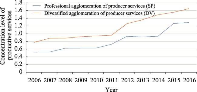
Fig. 3 Broken line chart of average level changes of producer services agglomeration in 286 cities in China
Table 6 Common trend test of producer service agglomeration and urban productivity change
Variable lnSPt-1 lnDVt-1 lnSPt-2 lnDVt-2 lnSPt-3 lnDVt-3 lnSPt-4 lnDVt-4 lnSPt-5 lnDVt-5 lnSPt-6 lnDVt-6
lnCP 0.016
(0.041)
0.009
(0.033)
0.014
(0.037)
0.011
(0.062)
0.014
(0.077)
0.012
(0.069)
0.017
(0.045)
0.011
(0.043)
0.017
(0.053)
0.013
(0.057)
0.019
(0.080)
0.013
(0.064)

5 Main conclusions and policy implications

Using the Moran index and the Lisa cluster diagram, this study analyzes the spatial correlation and distribution pattern of producer services agglomeration and productivity in Chinese cities from 2008 to 2018, and further empirically tests the effect of producer services agglomeration on urban productivity in China by using a spatial econometric model. The results of spatial data analysis show that there is a significant spatial autocorrelation between the agglomeration degree and productivity level of urban producer services in China, and they have obvious similarity and synchronization in their spatial distributions. The empirical results show that the level of urban productivity in Chinese cities is not only impacted by the productivity of neighboring cities, but also by the structural differences of the urban market scale, scientific and technological innovation investment, foreign direct investment, human capital and infrastructure level. On the whole, the technological externalities of producer services through specialized agglomeration and diversified agglomeration have significantly improved China’s urban productivity, but the “Marshall technological externalities” produced by the specialized agglomeration of producer services are more obvious. There are obvious differences in the impacts of producer services agglomeration on urban productivity in the eastern, central, western and northeastern regions of China. Among them, the technology spillover effect of producer services specialization agglomeration is greater in the cities of the eastern region and less prominent in the cities of the other three regions. The diversified agglomeration of producer services has a more obvious effect on the improvement of urban productivity in the western, central and northeastern regions, but has less effect on the cities in the eastern region.
The research conclusions provide important enlightenment for the discussion of reasonably arranging the urban industrial layout and promoting high-quality economic growth in the process of new urbanization construction in China.
In the process of transformation and upgrading of the economic growth mode, cities should pay attention to the technology spillover effect caused by the agglomeration of producer services. The state should strive to promote the agglomeration of producer services in central cities, and focus on improving their innovation and radiation capacity. At the same time, it should coordinate the technology spillover effects caused by the specialization and diversification of producer services in central cities, optimize the urban industrial structure with the agglomeration of producer services, and promote the simultaneous development of population urbanization and spatial urbanization. Such efforts would provide new impetus for improving urban productivity.
The professional agglomeration of producer services is an important factor for promoting the improvement of urban productivity, and plays a more obvious role in the improvement of eastern cities. Therefore, the eastern coastal cities, especially large cities such as Shanghai and Shenzhen, should actively develop highly specialized producer services to meet the demand for producer services in the transformation and development of the manufacturing industry. At the same time, they should use their radiation capacity to drive the development of producer services in the surrounding small and medium-sized cities. The cities in the other three regions should focus on the development of diversified producer services, create a good market competition atmosphere, and drive the improvement of urban productivity with the diversified agglomeration of producer services.
[1]
Andersson M. 2006. Co-location of manufacturing and producer service:A simultaneous equation approach. Working paper series in economics and institutions of innovation. London, UK: Routledge Press.

[2]
Anselin L. 1988. Spatial econometrics: Methods and models. Dordrecht, Netherlands: Kluwer Academic Publishers: 32-45.

[3]
Chen R. 2021. Study on the impact of producer services agglomeration and city size on urban productivity. Enterprise Economics, (8): 138-146. (in Chinese)

[4]
Chen S Y, Zeng L, Li W H. 2017. Local government competition, land transfer and urban productivity—Empirical evidence from 281 prefecture level cities in China. Financial Science, (7): 108-121. (in Chinese)

[5]
Chen X F, Zhou J J. 2020. Producer services agglomeration, spatial spillover and urban green total factor productivity—Empirical evidence from urban agglomeration in the Yangtze River Delta. Economic Longitude and Latitude, (4): 89-98. (in Chinese)

[6]
Combes P P. 2000. Economic structure and local growth: France, 1984-1993. Journal of Urban Economics, 47: 329-355.

[7]
Elhorst J. 2010. Applied spatial econometrics: Raising the bar. Spatial Economic Analysis, 5(1): 9-28.

[8]
Ezcurra R, Pascual M,Rapun. 2006. Regional specialization in the European Union. Regional Studies, 40(6): 601-616.

[9]
Glaeser E, Kalial H D, et al. 1992. Growth in cities. Journal of Political Economy, 100(6): 1127-1152.

[10]
Hou X S, Zhang Z Y, et al. 2014. Research on the growth effect and action path of China’s economic structure. World Economy, (5): 88-111. (in Chinese)

[11]
Hu B, Yu Z R. 2021. Research on the heterogeneous impact of local fiscal pressure on urban productivity: An analysis based on the background of new urbanization. Financial Research, 47(6): 139-153. (in Chinese)

[12]
Jacobs J. 1969. The economy of cities. New York, USA: Vintage Press: 45-62.

[13]
James P L, Kelly P R. 2009. Introduction to spatial econometrics. Boca Raton, USA: CRC Press: 513-514.

[14]
Ke S Z, Zhao Y. 2014. Industrial structure, city size and urban productivity in China. Economic Research, 4: 76-88. (in Chinese)

[15]
Li J K, Zhang T B. 2018. Study on the hierarchical impact and asymmetric effect of FDI in China’s urban productivity growth. Industrial Economic Research, 95(4): 18-29. (in Chinese)

[16]
Li R R. 2019. Producer services agglomeration and urban productivity—Differentiated learning effect, selection effect and classification effect. Chanjing Review, 10(1): 22-37. (in Chinese)

[17]
Liu P L, Song Z. 2007. Performance of China’s service and manufacturing industry enterprises: An empirical analysis based on China’s first economic census. Economic Research, (1): 47-58. (in Chinese)

[18]
Liu X W. 2019. Service industry agglomeration, urban innovation and urban productivity. Journal of Shanxi University of Finance and Economics, 41(7): 62-76. (in Chinese)

[19]
LV K B, Ren Z C. 2017. New demographic dividend, development of producer services and urban productivity—An empirical study based on urban agglomeration in the Yangtze River Delta. Nanjing Social Sciences, (1): 31-38. (in Chinese)

[20]
Marshall A. 1961. Principle of economics: An introductory volume. London, UK: Macmillan Press: 89-105.

[21]
Xi P H, Liang R B, Xie Z F, et al. 2017. Fiscal pressure, overcapacity and supply side Reform. Economic Research, (9): 88-104. (in Chinese)

[22]
Xu Q Y. 2010. An empirical study on the interactive relationship between industry and service industry in Shanghai based on VAR model. Shanghai Economic Research, (2): 90-97. (in Chinese)

[23]
Zhang C. 2018. Population density, human capital and urban productivity stratification—An empirical study based on Chinese urban data. Journal of Humanities, (2): 43-52. (in Chinese)

[24]
Zhang J, Wu G Y, Zhang J P. 2004. Estimation of China’s inter provincial physical capital stock: 1952-2000. Economic Research, (10): 35-44. (in Chinese)

[25]
Zhang S Q, Zhang P. 2017. The impact of innovation factor agglomeration and public expenditure on urban productivity—An empirical study based on the spatial panel of Beijing-Tianjin-Hebei-Mongolia. East China Economic Management, 31(11): 65-70. (in Chinese)

[26]
Zhang S Y, Wang C X, Ren Y J. 2019. Spatial spillover effect of producer services agglomeration on green total factor productivity. Soft Science, (11): 11-15, 21. (in Chinese)

[27]
Zhou Y, Tan G R. 2016. Research on the impact of producer services agglomeration on urban land intensive use from a spatial perspective. China Land Science, 30(10): 37-46. (in Chinese)

Outlines

/