Land Resource and Land Use

Delimiting Ecological Space and Simulating Spatial-temporal Changes in Its Ecosystem Service Functions based on a Dynamic Perspective: A Case Study on Qionglai City of Sichuan Province, China

  • OU Dinghua , 1, 2 ,
  • WU Nengjun 1 ,
  • LI Yuanxi 1 ,
  • MA Qing 1 ,
  • ZHENG Siyuan 1 ,
  • LI Shiqi 1 ,
  • YU Dongrui 1 ,
  • TANG Haolun 1 ,
  • GAO Xuesong , 1, 2, *
Expand
  • 1. College of Resources, Sichuan Agricultural University, Chengdu 611130, China
  • 2. Key Laboratory of Investigation and Monitoring, Protection and Utilization for Cultivated Land Resources, Ministry of Natural Resources, Chengdu 611130, China
* GAO Xuesong, E-mail:

OU Dinghua, E-mail:

Received date: 2021-05-24

  Accepted date: 2022-01-05

  Online published: 2022-10-12

Supported by

The Sichuan Science and Technology Program(2020YFS0335)

The Sichuan Science and Technology Program(2021YFH0121)

The National College Students' Innovative Entrepreneurial Training Plan Program of Sichuan Agricultural University(202110626038)

The Double Support Program Project of Discipline Construction of Sichuan Agricultural University of China(2018)

The Double Support Program Project of Discipline Construction of Sichuan Agricultural University of China(2019)

The Double Support Program Project of Discipline Construction of Sichuan Agricultural University of China(2020)

Abstract

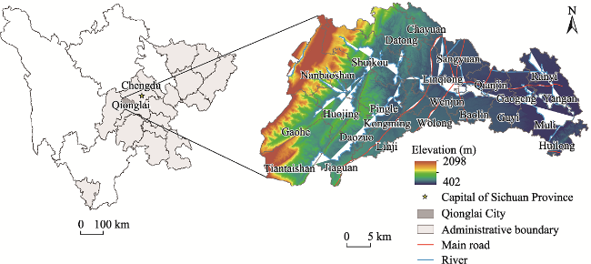
Delimiting ecological space scientifically and making reasonable predictions of the spatial-temporal trend of changes in the dominant ecosystem service functions (ESFs) are the basis of constructing an ecological protection pattern of territorial space, which has important theoretical significance and application value. At present, most research on the identification, functional partitioning and pattern reconstruction of ecological space refers to the current ESFs and their structural information, which ignores the spatial-temporal dynamic nature of the comprehensive and dominant ESFs, and does not seriously consider the change simulation in the dominant ESFs of the future ecological space. This affects the rationality of constructing an ecological space protection pattern to some extent. In this study, we propose an ecological space delimitation method based on the dynamic change characteristics of the ESFs, realize the identification of the ecological space range in Qionglai City and solve the problem of ignoring the spatial-temporal changes of ESFs in current research. On this basis, we also apply the Markov-CA model to integrate the spatial-temporal change characteristics of the dominant ESFs, successfully realize the simulation of the spatial-temporal changes in the dominant ESFs in Qionglai City's ecological space in 2025, find a suitable method for simulating ecological spatial-temporal changes and also provide a basis for constructing a reasonable ecological space protection pattern. This study finds that the comprehensive quantity of ESF and its annual rate of change in Qionglai City show obvious dynamics, which confirms the necessity of considering the dynamic characteristics of ESFs when identifying ecological space. The areas of ecological space in Qionglai city represent 98307 ha by using the ecological space identification method proposed in this study, which is consistent with the ecological spatial distribution in the local ecological civilization construction plan. This confirms the reliability of the ecological space identification method based on the dynamic characteristics of the ESFs. The results also show that the dominant ESFs in Qionglai City represented strong non-stationary characteristics during 2003-2019, which showed that we should fully consider the influence of the dynamics in the dominant ESFs on the future ESF pattern during the process of constructing the ecological spatial protection pattern. The Markov-CA model realized the simulation of spatial-temporal changes in the dominant ESFs with a high precision Kappa coefficient of above 0.95, which illustrated the feasibility of using this model to simulate the future dominant ESF spatial pattern. The simulation results showed that the dominant ESFs in Qionglai will still undergo mutual conversions during 2019-2025 due to the effect of the their non-stationary nature. The ecological space will still maintain the three dominant ESFs of primary product production, climate regulation and hydrological regulation in 2025, but their areas will change to 32793 ha, 52490 ha and 13024 ha, respectively. This study can serve as a scientific reference for the delimitation of the ecological conservation redline, ecological function regionalization and the construction of an ecological spatial protection pattern.

Cite this article

OU Dinghua , WU Nengjun , LI Yuanxi , MA Qing , ZHENG Siyuan , LI Shiqi , YU Dongrui , TANG Haolun , GAO Xuesong . Delimiting Ecological Space and Simulating Spatial-temporal Changes in Its Ecosystem Service Functions based on a Dynamic Perspective: A Case Study on Qionglai City of Sichuan Province, China[J]. Journal of Resources and Ecology, 2022 , 13(6) : 1128 -1142 . DOI: 10.5814/j.issn.1674-764x.2022.06.017

1 Introduction

Ecological space is a complex geographical space composed of multiple ecosystems, with the main functions of providing ecological products or ecological services (Chen et al., 2020; Gao et al., 2020). Ecosystem service functions (ESFs) are the natural environmental conditions and their utility formed by ecosystems and ecological processes to maintain human survival (Daily, 1999; Daily et al., 2000). They have spatial-temporal dynamics (Shi et al., 2012) and multifunctionality (Costanza et al., 1997), which often make the ecological space present similar characteristics. Moreover, there must be a function that plays a dominant role among the various ESFs within a certain ecological space. Therefore, demarcating ecological space from the perspective of spatial-temporal dynamics of the ESFs and simulating the spatial pattern in the future of the dominant ESFs for ecological space according to the spatial-temporal change characteristics of the dominant ESFs may have important theoretical and practical significance for scientifically demarcating the ecological conservation redline and ecologically controlled area, constructing and optimizing the national ecological security pattern, ensuring regional ecological security and promoting the high-quality development of the economy and society.
With the deepening of the national ecological civilization construction strategy, some practitioners and theoretical researchers have conducted many useful explorations around the identification (demarcation) of ecological space. In practice and application, relevant ministries and commissions of the PRC have issued guiding documents such as the National Ecological Function Zoning and the Guidelines for the Delimiting of the ecological conservation redline, which laid a foundation for local governments to carry out the demarcation of ecological space and construct the regional ecological security patterns. However, these practices hardly ever consider the spatial-temporal dynamics of the ESFs and their dominant functions. In the theoretical research, many ecological space identification studies have focused on the methods, which mainly included qualitative research related to directly demarcating ecological space based on land use/cover type (Li et al., 2016; Zhang et al., 2016), and quantitative research on demarcating ecological space by integrating the importance of ESFs and the sensitivity of the ecological environment (Xie et al., 2018; Xu et al., 2020). Similar to the practice and application, these theoretical studies on ecological space identification are mostly static and rarely consider the spatial-temporal dynamics of ESFs.
Numerous models (methods) have emerged in the field of spatial change simulation, benefiting from the development of computer technology. The common models include cellular automata (CA) model (Moreno et al., 2008; Al-Ahmadi et al., 2009), the conversion of land use and its effect on small regional extent (CLUE-S) model (Zhou et al., 2016; Kucsicsa et al., 2019), linear programming model (Kumar et al., 2016; Ma and Zhou, 2018) and Markov chain (Al-sharif and Pradhan, 2014; Pahlavani et al., 2017). The CLUE-S and CA models are good at spatial change simulation and can reflect spatial dynamic changes well, but there are certain limitations in their quantitative structure simulations. The linear programming model and Markov chain can realize quantitative change predictions well, but have difficulty with simulating spatial change. Therefore, the composite models integrating quantitative structure and spatial pattern simulation, such as Markov-CA (Halmy et al., 2015), DE-CA (Wang et al., 2015), and PSO-CA (Feng et al., 2011), have been widely used in the field of spatial change simulation, including land use and urban expansion, whereas they have seldom been applied in the simulation of spatial-temporal changes of ecological space, and it is even more rare to directly apply them to the simulation of spatial-temporal changes of the dominant ESFs in ecological space. For a long time, the simulation of ecological space changes has mainly focused on the analysis of ecological space evolution (Guan et al., 2013; Yao et al., 2015). In the past two years, a few studies have used composite models to simulate ecological spatial changes (Wang et al., 2020). Therefore, it is a useful exploration to simulate spatial-temporal changes in the dominant ESFs of ecological space by applying the composite models.
Although scholars have made rich achievements in the research fields related to ecological space identification and the simulation of its dominant ESF changes, there are still some deficiencies and omissions. Firstly, the ecological space has been delimited mostly by the current ecosystem structure and service function status, while ignoring the spatial-temporal dynamics of the ecological space because of the evolution of its ESFs, so the reliability of the resulting ecological space identification is low. Secondly, the analysis of ecological space evolution mostly focuses on quantitative and spatial changes, while ignoring the spatial-temporal change analysis of the dominant ESFs in ecological space, and fails to provide reliable foundation support for constructing the ecological space protection pattern. Thirdly, the composite models integrating the quantitative structure and spatial pattern have been applied rarely to the simulation of the changes in the dominant ESFs in the ecological space, and the theoretical research results are relatively weak.
Our goal in this paper is to propose a new ecological space identification method based on the dynamic change characteristics of the ESFs and to try to integrate the Markov-CA model with the spatial-temporal change characteristics of the dominant ESFs to simulate the spatial-temporal change in the dominant ESFs in the ecological space, with the aim of solving the deficiencies of the research in related fields. To do this, we 1) delimited the ecological space based on the spatial-temporal dynamic characteristics of the comprehensive ESFs during 2003-2019; 2) identified the dominant ESFs of the ecological space and analyzed their change characteristics; and 3) simulated the dominant ESF spatial pattern of the ecological space in 2025 with the Markov-CA composite model. The general intent of this work is to provide a theoretical basis and method reference for reasonably delimiting the ecological conservation redline, optimizing the ecological space protection pattern and realizing sustainable development.

2 Materials and methods

2.1 Study area

Qionglai City is located in the central portion of Sichuan Province, between 30°12'N-30°33'N and 103°04'E- 103°45'E, which is at the transition zone of the Chengdu Plain and the Longmen Mountains. The city's total area is 1377 km2, covering 1 neighborhood, 19 towns, and 4 townships (Fig. 1). Its terrain gradually slopes from the northwest to the southeast, with the highest elevation of 1991 m and the lowest elevation of 451 m. There are plains, moun tains, hills and other landform types. Among them, the area of plains is 311.36 km2, distributed in the east and northeast of the territory. The area of mountains is 817.79 km2, with the Wumianshan, Changqiu mountainous area in the south, and the extended mountain system of the southern section of Longmen Mountain in the west. The area of hills is 245.98 km2, with a dispersed distribution in the northwestern margin of the central part of the study area. The study area is rich in water resources, and rivers passing through the territory are 271.25 km long. Qionglai City is a subtropical moist zone, with an average annual temperature of 16.3 ℃, rainfall of 1117.3 mm, sunshine hours of 1107.9 h, and a perennial average evaporation of 1024.92 mm. The main soil types are alluvial soil and purple soil. The forest vegetation type is subtropical evergreen broad-leaved forest, which is mainly distributed in the northwest of the middle-low mountains and central hilly areas. Qionglai City is the new center of the west in the state-level Tianfu New Area focusing on the development of ecological and tourism industries, and its GDP reached 33.073 billion yuan in 2020.
Fig. 1 Geographical location of the study area
(from the Resource and Environmental Science Data Center of the Chinese Academy of Sciences http://www.resdc.cn/).

2.2 Data sources and processing

The basic study data are the land use data of Qionglai City in odd years during 2003-2019. The land use data for 2009 are from the second national land survey of Qionglai City, classifying the land according to “the GBT 21010-2007 Current Land Use Classification”. The land use data for 2011, 2013, 2015, 2017, and 2019 are the annual land use change survey data of Qionglai City, which adopt the same classification system as the data for 2009. Land use data for 2003, 2005 and 2007 were obtained by using ESRI ArcGIS to modify patches on the land use map for 2009 that have changed by referring to high-definition Google satellite images (obtained by 91 Satellite Assistant) in the corresponding years. In addition, in order to determine the regional vegetation types, we also referred to the spatial distribution data of China's 1:1 million vegetation types Due to the inconsistent coordinates of the land use, satellite imagery, and vegetation type data, we first unified the geographic coordinates of the data into WGS-84 coordinates and the projection into a UTM projection by ESRI ArcGIS. At the same time, we transformed the land use vector data into raster data with a unified raster size of 100 m×100 m. Then, we divided the ecosystem types of Qionglai City into seven categories: farmland, forest, grassland, wetland, waters, desert, and settlement, by referring to authoritative research results (Costanza et al., 1997; Xie et al., 2010; Xie et al., 2015) and combining it with the status of the regional ecosystem. Lastly, we merged the preliminary processed land use raster data according to the corresponding relationship shown in Table 1 with the support of ESRI ArcGIS, so that the ecological system type distribution raster data of Qionglai City during 2003-2019 were obtained.
Table 1 Correspondence between ecosystem types and land use types
Ecosystem type Land use type
Cropland Paddy filed, irrigated cropland, rainfed cropland
Forest land Woodland, shrubbery land, other woodlands, fruit plantation, tea plantation, other orchards
Grassland Other grasslands
Wetland Inland mudflat
Water body River, pond, reservoir, ditches
Desert Sand, barren land
Settlement Mining land, land for scenic site facilities, railway, highway, rural road, city, organic town, village, hydraulic structure, land for agricultural facilities

2.3 Research methods

2.3.1 Dynamic identification of ecological space

The processes of ecological space identification considering the spatial-temporal dynamics of ecosystem service functions includes three steps.
(1) Establish the evaluation units of ESFs for ecological space. The grid cells are used as the evaluation units, and their size is closely related to the evaluation scale. Due to the obvious scale effect of ecological space (Gao et al., 2019), the grid is so small that it will lose macro variation characteristics and increase data redundancy, otherwise it will ignore fine- scale changes and reduce the accuracy of the results. The grid size of the evaluation units was determined to be 100 m×100 m after referring to the Guidelines for the Demarcation of Ecological Protection Red Line and comprehensively considering the study area scope and the amount of data operations. Then, we constructed the grid vector data of the evaluation units for the ESFs of the ecological space with the support of ESRI ArcGIS Create Fishnet tool. There were 139738 grid units in the study area.
(2) Calculate the ESF quantity of the evaluation unit. The methods of accounting ESF values mainly include the function value method (Zhao et al., 2004) and equivalent factor method (Xie et al., 2008). Of these methods, the equivalent factor method has the characteristics of simple application and easy comparability of results, which is suitable for the spatial-temporal dynamic evaluation of the ecosystem service function value (Costanza et al., 2014; Wang et al., 2014). The purpose of this study is to delimit the ecological space and simulate its evolutionary trend based on ESFs and their change characteristics. If the ESF quantity is converted into economic value (Xie et al., 2003, 2008, 2015), it may not be able to accurately reveal the change characteristics of the ESF quantity due to the instability of grain yield and price fluctuations (Under the influence of uncertain factors such as market supply and demand relationships and government macro-control policies, grain prices fluctuate frequently). Therefore, the equivalent of ecosystem service value can be directly used as a “measurement” of the ESF quantity. The steps for evaluating the ESF quantity of the evaluation unit are as follows:
First, the equivalent of ecosystem service value per unit area is determined. We constructed the ecosystem types and their ESF systems according to the basic equivalence table of ecosystem service value per unit area (equivalent table) (Xie et al., 2015), and combined it with the actual ecosystem types and land use types in Qionglai City. Among them, the ecosystem types were divided into one layer and seven categories, which included farmland (corresponding to dry land and water field in the equivalent table), forest (corresponding to coniferous forest, broad-leaved forest, and shrubbery in the equivalent table), grassland (corresponding to grassland, scrub-grass-land, and meadow in the equivalent table), wetland (corresponding to wetland in the equivalent table), desert (corresponding to desert and bare land in the equivalent table), waters (corresponding to the water system in the equivalent table), and seven types of settlements. The ESF types were divided into four primary categories: provisioning service, regulation service, supporting service, and cultural service. The provisioning service included a secondary category: primary product production, which corresponded to the production of food and raw materials in the equivalent table. The regulation service included four secondary categories: gas regulation, climate regulation, hydrological regulation, and environmental purification; and the hydrological regulation corresponded to the water supply and hydrological regulation in the equivalent table. The supporting service included two secondary categories: soil conservation and biodiversity conservation; and the soil conservation corresponded to soil conservation and nutrient cycling in the equivalent table. The cultural service included one secondary category, which was completely consistent with the equivalent table. We calculated the equivalent ecosystem service value per unit area in the equivalent table according to the aforementioned corresponding relationship, and then obtained the equivalent of ESF per unit area for each ecosystem in Qionglai City (Table 2).
Table 2 Equivalence of ecosystem service values supplied per unit area
Ecosystem type Provision service Regulation service Support service Cultural service
PPP GR CR EP HR SC BIO AL
Farmland 1.35 0.89 0.47 0.14 0.19 0.68 0.17 0.08
Forest 0.77 1.76 5.27 1.57 4.09 2.31 1.95 0.86
Grassland 0.58 1.21 3.19 1.05 2.53 1.58 1.34 0.59
Wetland 1.01 1.90 3.60 3.60 26.82 2.49 7.87 4.73
Desert 0.00 0.02 0.00 0.10 0.03 0.02 0.02 0.01
Waters 1.03 0.77 2.29 5.55 110.53 1.00 2.55 1.89
Settlement 0.00 0.00 0.00 0.00 0.00 0.00 0.00 0.00

Note: PPP, GR, CR, EP, HR, SC, BIO, AL represent primary product production, gas regulation, climate regulation, environmental purification, hydrological regulation, soil conservation, biodiversity, and aesthetic landscape, respectively.

We then calculated the ESF quantity. We determined the area of each type of ecosystem in the evaluation unit using the Tabulate Area tool of ESRI ArcGIS and calculated each ESF quantity such as primary product production and gas regulation according to Eq. (1), and lastly calculated the comprehensive ESF quantity of the evaluation unit according to Eq. (2).
${{V}_{{k}'j}}=\underset{l=1}{\overset{M}{\mathop \sum }}\,{{\upsilon }_{lj}}{{s}_{{k}'l}}$
${{V}_{{{k}'}}}=\underset{j=1}{\overset{n}{\mathop \sum }}\,{{V}_{{k}'j}}=\underset{j=1}{\overset{n}{\mathop \sum }}\,\underset{l=1}{\overset{M}{\mathop \sum }}\,{{\upsilon }_{lj}}{{s}_{{k}'l}}$
where ${{\upsilon }_{lj}}$ is the equivalent of the j-th ESF of the l-th type of ecosystem. ${{s}_{{k}'l}}$ is the area of the l-th type of ecosystem in the ${k}'$-th evaluation unit. ${{V}_{{k}'j}}$, ${{V}_{{{k}'}}}$ are the quantity and comprehensive quantity of the j-th ESF of the ${k}'$- th evaluation unit, respectively. $M,n$ are the number of ecosystem types and the number of ESF types, respectively. $i,j,{k}'$ are the ecosystem types, ESF types, and evaluation unit number, respectively; where $l=1,2,\cdots,M;j=1,2,\cdots,n;{k}'=1,2,\cdots,K$, K is the number of evaluation units.
(3) Identify the ecological space. Because of the spatial-temporal heterogeneity of ecological space (Costanza et al., 2014; Wang et al., 2014), the ecological space defined by conventional methods (i.e., according to the needs of regional ecological protection and the reality of ecological construction, the regions with current ESF quantity greater than a certain threshold value are divided into ecological space) may not provide the best ecological security guarantee for the region in the future. Usually, the ecological space with frequent changes is more likely to be disturbed by human beings, and the stability of its ESFs is poor, so identifying it as ecological space is bound to reduce the regional ecological security degree. On the contrary, the ecological space with a small range of changes is less likely to be disturbed by human beings, so the structure and function of its ecosystem are more stable, and the protection of the regional ecological security is more reliable, thus it should be identified as ecological space. Therefore, based on the analysis of changes in the comprehensive ESFs in a long time series, the units with a comprehensive ESF quantity greater than or equal to a certain threshold and with an average change rate less than or equal to a certain threshold are delimited as ecological space. The mathematical expression is:
$\begin{align} & E=\left\{ {{e}_{1}},{{e}_{2}},\cdots,{{e}_{k}},\cdots,{{e}_{m-1}},{{e}_{m}} \right\}= \\ & \left\{ {{e}_{k}}\text{ }\!\!|\!\!\text{ }V_{k}^{t}\ge \delta,\frac{1}{T-1}\underset{t=2}{\overset{T}{\mathop \sum }}\,\left| \frac{V_{k}^{t}-V_{k}^{t-1}}{V_{k}^{t-1}} \right|\le \varepsilon \right\} \\ \end{align}$
where E is ecological space. ek is the vector grid that composes E. $V_{k}^{t}$ is the comprehensive ESF quantity of unit k in year t, and its calculation method is shown in Eq. (2). k, m represent the code and number of grids that make up E, respectively. t, T represent any time section and the number of time sections, respectively. $\delta,\varepsilon $ represent quantities of the comprehensive ESF and its change rate for dividing the ecological space and the non-ecological space, respectively, which are determined by the standard deviation grading method. In this study, the grid with a comprehensive ESF quantity of nine time sections in odd years during 2003–2019 not less than δ and an annual change rate not greater than $\varepsilon $ was identified as ecological space, otherwise it was non-ecological space.

2.3.2 Change analysis of the dominant ESFs of the


ecological space
The dominant ESFs have obvious spatial-temporal dynamic characteristics, and the processes and steps in the analysis of the evolution characteristics are as follows:
(1) Identification of the dominant ESFs in the ecological space. Taking the vector grid cells as the identification units, the ESF type with the largest quantity was taken as the dominant ESF of the grid cell, and taken collectively, they revealed the dominant ESF pattern of the ecological space. The mathematical expression is as follows:
$\begin{align} & D=\left\{ d_{1}^{{{j}_{1}}},d_{2}^{{{j}_{2}}},\cdots,d_{k}^{{{j}_{k}}},\cdots,d_{m-1}^{{{j}_{m-1}}},d_{m}^{{{j}_{m}}} \right\}= \\ & \left\{ d_{k}^{{{j}_{k}}}\text{ }\!\!|\!\!\text{ }{{V}_{k{{j}_{k}}}}=\text{max}\left\{ {{V}_{k1}},{{V}_{k2}},\cdots,{{V}_{kj}},\cdots,{{V}_{k,n-1}},{{V}_{kn}} \right\} \right\} \\ \end{align}$
where D is the dominant functional pattern of ecological space. $d_{k}^{{{j}_{k}}}$ is the ESF of the k- $\text{th}$ grid cell, whose number is ${{j}_{k}}\in [n]$, and the codes 1, 2, 3, 4, 5, 6, 7, and 8 represent primary product production, gas regulation, climate regulation, environmental purification, hydrological regulation, soil conservation, biodiversity and aesthetic landscape functions, respectively. ${{V}_{k{{j}_{k}}}}$ is the quantity of the dominant ESF jk of the k-th grid cell; Vkj is the j-th ESF quantity of the k-th grid cell; $k,m$ have the same meanings as in Eq. (3); and $j,n$ have the same meanings as in Eq. (2).
(2) Analysis of the evolution of the dominant ESFs in the ecological space. We used the IDRISI software Markov module to calculate the transition probability matrix of the dominant ESFs in 2003-2007, 2007-2013 and 2013-2019, based on the grid maps of the dominant ESFs of the ecological space in 2003, 2007, 2013 and 2019; and then analyzed the change characteristics of the quantitative structure of the dominant ESFs in each stage. Meanwhile, we acquired the spatial distribution of the dominant ESF change types in the ecological space in 2003-2007, 2007-2013 and 2013-2019 with the support of ESRI ArcGIS analysis tool. Then, we analyzed the spatial change characteristics of the dominant ESFs in each stage.

2.3.3 Simulation of the changes in the dominant ESFs of the ecological space

Simulating the spatial pattern of the dominant ESFs of the ecological space in 2025 by using the Markov-CA composite model. The main processes and steps are as follows:
(1) Define model parameters. We defined the cell as the grid of the distribution of the dominant ESFs (the size of the grid is 100 m), defined the cellular space as the spatial pattern of the dominant ecosystem service functions, defined the cell state as eight types of ESFs: primary product production, gas regulation, climate regulation, environmental purification, hydrological regulation, soil conservation, biodiversity and aesthetic landscape, and used a standard 5×5 proximity filter.
(2) Verify the model accuracy. Firstly, based on the grid maps of the dominant ESFs in 2007, 2011, 2013, 2015, and 2017 selected by the evolutionary characteristics of the dominant ESFs in the ecological space and the needs of simulation data, we applied the Markov model to calculate the transition probability matrix and conditional probability map of the dominant ESFs in 2015-2017, 2011-2015 and 2007-2013 with the support of the IDRISI software, which were respectively used as the cellular number and spatial transformation rules of CA (Sang et al., 2011). Then, based on the defined parameter in Step 1 and the cellular number and spatial transformation rules of the three aforementioned periods, we applied the Markov-CA module of the IDRISI software to simulate the dominant ESFs in 2019, respectively. Finally, we calculated the Kappa coefficients of the simulated and actual distribution maps of the dominant ESFs in 2019 separately to evaluate the model accuracy. The model could be used to simulate the spatial changes when the consistency between the simulated distribution map and the actual distribution map was moderate or above; otherwise, we should adjust the model parameters or simulation data and re-check the accuracy until it meets the accuracy requirements.
(3) Apply the simulation models. When the model accuracy is qualified, we could select the grid maps of the dominant ESFs in 2013 and 2019 according to the timehomogeneity and no aftereffect of the Markov chain and the time interval of the accuracy test data of the model. Then we could construct the cell number and space transformation rules, and set the model parameters by referring to the steps in (2). After that, the layout of the dominant ESFs of the ecological space in 2025 were simulated by using the Markov-CA module of the IDRISI software.

3 Results and analysis

3.1 Change characteristics of the comprehensive ESFs and analysis of the results for delimiting ecological space

3.1.1 Change characteristics of the comprehensive ESFs

The standard deviation classification method was used to classify the comprehensive ESF quantity in Qionglai in the odd years from 2003 to 2019. These classification results showed that the grading number of the comprehensive ESF quantity was different in each year, but the classification thresholds showed a strong consistency (Fig. 2). Among these classification results, the first classification thresholds are 6.88, 6.84, 6.86, 6.96, 6.84, 6.78, 6.67, 6.66, and 6.65 for each of the years, respectively, whose standard deviation is 0.1042. This indicates that the first classification thresholds have limited fluctuations and are relatively stable. In addition, Qionglai is an important part of building a regional ecological security pattern, and it is a national demonstration county for ecological civilization construction and belongs to the main area of Chengdu “West Control” Strategic Master Plan (2017-2035). Therefore, the average of the first classification thresholds for the comprehensive ESF quantity value in each year (6.79) was taken as the critical value of the comprehensive function quantity for dividing the ecological space and non-ecological space in Qionglai. (Note that in practice, the second, third or other thresholds can also be used as the critical value of the comprehensive function quantity for dividing ecological space and non-ecological space based on the actual situation of the region.) Moreover, the regions with a comprehensive ESF quantity greater than 6.79 are mainly distributed in the western mountainous area, the river basin and the shallow hilly area in the central and southern parts of the area, where the ecological resources are rich and the vegetation coverage is high. Thus, it is consistent with common sense and the regional reality to delimit these areas as ecological space (Fig. 3c).
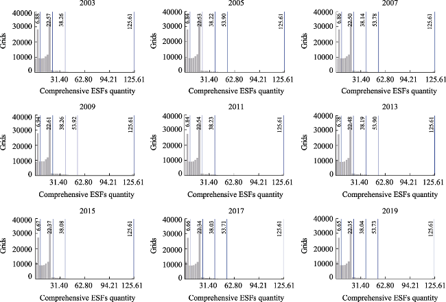
Fig. 2 Standard deviation grading chart for the comprehensive ESF quantity in Qionglai during 2003-2019
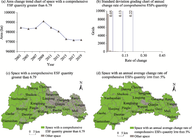
Fig. 3 The process map of ecological space identification in Qionglai
However, the spatial area with a comprehensive ESF quantity greater than 6.79 in each year fluctuated greatly, showing a trend of increasing at first and then decreasing (Fig. 3a). Generally, it is not suitable to demarcate the ecological space with frequent changes as ecological space because it is greatly disturbed by human beings, and the stability of its ESF is poor. Therefore, if all areas with a comprehensive ESF quantity greater than 6.79 are demarcated as ecological space, it would inevitably reduce the degree of regional ecological security. In conclusion, when we demarcate the ecological space, the change characteristics of the comprehensive ESF quantity should also be considered to enhance the stability of ecological space identification. For this reason, this study applied the standard deviation grading method to classify the average annual change rate of the comprehensive ESF quantity. As a result, there were four classification thresholds of 5%, 13%, 22%, 34.4% (Fig. 3b). Theoretically, the area with a comprehensive ESF quantity $~\ge \delta $ and which remains unchanged, i.e., its average annual change rate is 0, is the most stable ecological space. Actually, due to the complexity of the ecosystem itself and the inevitable errors in data analysis, there are few areas where the value is absolutely unchanged. So, the first classification threshold of 5% for the annual average change rate of the comprehensive ESF quantity was used as the comprehensive function change rate critical value for differentiating the ecological space and non- ecological space in Qionglai City. Moreover, in terms of the spatial pattern, the areas with an average annual change rate of the comprehensive ESF quantity less than 5% are mainly distributed in the western mountainous areas and the central shallow hilly areas, which are relatively less disturbed by human activities, so it is also consistent with common sense and the regional reality to allocate these areas to the ecological space (Fig. 3d).

3.1.2 Analysis of the results for delimiting the ecological space

An area with a comprehensive ESF quantity greater than 6.79 (Fig. 3c) and an annual average change rate of less than 5% (Fig. 3d) should be delimited as an ecological space, comprehensively considering the impact of the ESFs and the change rate of the ecological space (Fig. 4). The total area of ecological space in Qionglai is 98307 ha, accounting for 71.39% of the total land area. The ecosystem types in the ecological space are mainly woodland, farmland and waters, accounting for 65.14%, 24.56% and 4.57% of the total ecological space, respectively. The ecological space is concentrated and contiguously distributed in the western mountainous areas and slightly scattered in the eastern dam areas such as Chayuan, Kongming, Wolong, Baolin, Guyi, Huilong and the west of Linqiong. The ecological space is concentrated in these areas because the western and southern parts of the city are mainly mountainous and shallow hilly landforms, where the forests are distributed in patches and the ESFs are high and stable. The eastern part is mostly non-ecological space because it is a dam area with vertical and horizontal water systems, dense populations, well-developed transportation, frequent human activities, and great disturbance to the ecosystem, so the ecosystem service function value is relatively low and changes frequently in this area.
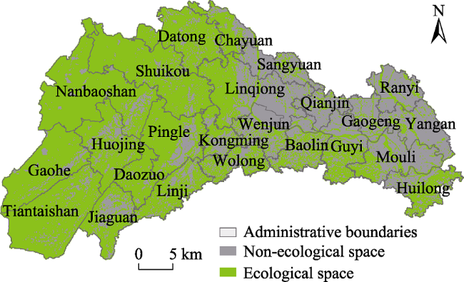
Fig. 4 The map of ecological space (comprehensive function quantity≥6.79 and annual change rate≤5%) identification in Qionglai

3.2 Analysis of the change characteristics of the dominant ESFs of the ecological space during 2003‒2019

3.2.1 Quantitative structural change characteristics of the dominant ESF

The dominant ESF types in ecological space all changed significantly, among which the transfers of “primary product production → climate regulation”, “climate regulation → primary product production”, and “hydrological regulation → primary product production” were the most conspicuous during the period of 2003-2019 (2003-2007, 2007-2013, and 2013-2019) (Table 3). In terms of the transfer of dominant ESFs, the functional areas of primary product production were transferred out of 244 ha, 258 ha, and 542 ha, respectively, in the three periods, which were mainly converted to climate regulation, accounting for 79.92% (36.11%), 75.19% (20.74%), 83.03% (33.86%) of the transfer area of primary product production in each period (i.e., the total transfer area of the dominant ESFs). The functional areas of climate regulation were transferred out of 215 ha, 603 ha, and 637 ha, respectively, which were mainly converted to primary product production, accounting for 93.02% (37.04%), 99.17% (63.62%), 95.13% (45.60%) of the transfer area of climate regulation (i.e., the total transfer area of the dominant ESFs). The transfer area of “climate regulation → primary product production” was much larger than the total area of primary product production function transferred out during the second period, which is why the “climate regulation → primary product production” is the dominant factor for the area increase in the primary product production functional areas. The transferred areas of hydrological regulation were relatively small in the first two periods, but it was significant in the third period. It was mainly converted into the primary product production, and the transfer area was 150 ha, accounting for 84.00% and 9.48% of the transfer areas of the hydrological regulation functional area and the dominant ESFs.
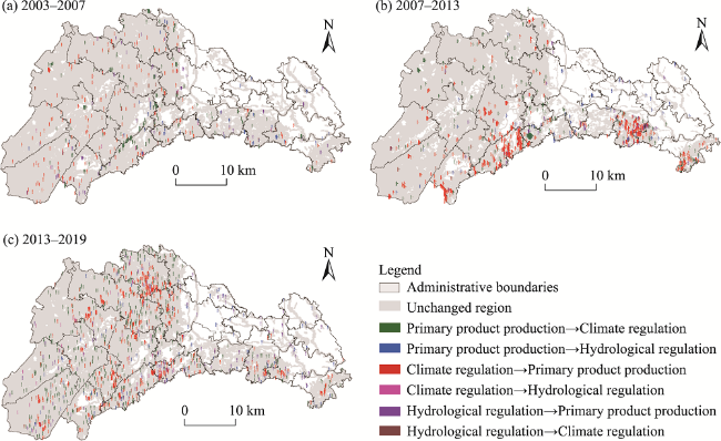
Table 3 The transfer area matrix of the dominant ESFs of the ecological space in Qionglai during 2003-2007, 2007-2013 and 2013-2019.
Function type 2003‒2007 2007‒2013 2013‒2019
PPP CR HR PPP CR HR PPP CR HR
PPP (ha) 29083 200 59 29084 598 65 29205 606 126
CR (ha) 195 55201 22 194 54815 14 450 54386 24
HR (ha) 49 15 13483 64 5 13468 92 31 13387

Note: The meanings of PPP, CR, HR is the same as Table 2.

3.2.2 Spatial layout change characteristics of the dominant ESFs

The spatial distribution of the “primary product production → climate regulation” showed consistency and continuity, and it was mainly distributed in the western mountainous areas during 2003‒2019. It was concentrated in the southwest of Wolong with the highest degree of agglomeration during 2007‒2013, and was scattered in the western mountainous area during 2013‒2019. The transfer type of “primary product production → climate regulation” was driven by the rugged terrain, dense forest, low traffic accessibility and low population density in the western mountainous areas, the increase of farmland abandoned by farmers, and the government's ecological protection policies such as returning farmland to forest (Fig. 5).
Fig. 5 Spatial distribution map of the change types of the dominant ESFs in Qionglai during 2003-2007, 2007-2013 and 2013-2019.
The change type of “climate regulation → primary product production” was distributed sporadically in the western mountainous area, with the smallest distribution range and the highest dispersion degree during 2003-2007. Its spatial distribution showed obvious agglomeration, which was mainly concentrated in Pingle, Linji, Jiaguan, the southwest of Guyi and Huilong, while the agglomeration degree in the southwest region was higher than that in the southeast region during 2007‒2013. It was mainly distributed in the southwestern and northwestern parts of the city, with a vast distribution range during 2013‒2019. This is because the southwestern and northwestern regions vigorously develop their tourism industry with rich tourism (e.g., AAAA-level scenic spots such as Tiantaishan National Forest Park and West Sichuan Bamboo Sea), and the human interference may affect the stability of the forest ecosystem functions. In addition, the needs for food security and farmland protection have led to the transfer of the climate regulation function to the primary product production functions (Fig. 5).
The change type of “hydrological regulation → primary product production” was concentrated in the central and southern parts of Wolong and Guyi, as well as the northwest of Datong county during 2013‒2019. This is because Qionglai continued to optimize and adjust the agricultural industrial structure and implemented moderate scale management in recent years. For example, according to the Control Plan of Urban Modern Agricultural Industry in Qionglai City, high-quality grain and oil bases would be concentrated in Guyi, Wolong and other towns, which would be kept at 60000 ha, including 4000 ha of high-end seed industry bases, 3333 ha of standardized and large-scale facility vegetable fields, 2667 ha of perennial vegetable bases and standardized kiwi bases until 2019. As a result, some ponds with small storage capacity and low development and utilization value in the area were adjusted to the corresponding agricultural industrial areas, which generated the transfer of hydrological regulation function to the primary product production functions (Fig. 5).

3.3 Analysis of the simulation results of the spatial changes in the dominant ESFs of the ecological space in 2025

3.3.1 Accuracy of simulating spatial changes in the dominant ESFs with the Markov-CA model

We adopted the Kappa coefficient classification standard put forward by Feinstein (Feinstein et al., 1990; Cicchetti et al., 1990) to evaluate the simulation effect of the model. In that system, when Kappa < 0.00, 0.01 < Kappa < 0.20, 0.21 < Kappa < 0.40, 0.41 < Kappa < 0.60, 0.61 < Kappa < 0.80, or 0.81 < Kappa < 1.00, these levels indicate that the consistency of the two images is insignificant, very weak, weak, moderate, significant or the best, respectively. The Kappa coefficients of the time gradient of 2, 4, and 6 years were 0.9737, 0.9730, and 0.9689, respectively, according to the calculation results (Table 4). This indicated that the consistency between the simulation results and the actual distribution decreased slowly with the increase of the gradient, but both of them reached the optimal level. So the results showed that the model is reliable and can be used to simulate the spatial changes in ESFs.
Table 4 The accuracy of simulating spatial changes in the dominant ESFs with the Markov-CA model
Basic data Time gradient Simulation (test) data Kappa coefficient
Distribution map of dominant ecosystem service functions in 2015 and 2017 2 Distribution map of dominant ecosystem service functions in 2019 0.9737
Distribution map of dominant ecosystem service functions in 2011 and 2015 4 Distribution map of dominant ecosystem service functions in 2019 0.9730
Distribution map of dominant ecosystem service functions in 2007 and 2013 6 Distribution map of dominant ecosystem service functions in 2019 0.9689

3.3.2 Analysis of the simulation results of the spatial changes in the dominant ESFs

In 2025, the ecological space will still maintain the three dominant ESFs of primary product production, climate regulation and hydrology regulation, whose areas will be 32793 ha, 52490 ha and 13024 ha, respectively, accounting for 33.36%, 53.39% and 13.25% of the total ecological space (Table 5). The functional areas of primary product production are concentrated in the southwest, northwest and central south, with others scattered in the western valley area (Fig. 6a). This region is to be delimited as functional area of primary product production because it is located in a mountain valley and central plain with good irrigation conditions, fertile soil and high primary product production capacity. The functional areas of climate regulation are concentrated in the western mountainous areas, and others are widely scattered in the southwest of Mouli and southeast of Huilong. It is sensible to delineate this area as a climate regulation functional area, because it is a concentrated forest distribution area, so the green plants can regulate atmospheric oxygen and carbon dioxide by respiration and photosynthesis, and forest plant evapotranspiration can also regulate the regional microclimate. The functional areas of hydrological regulation are mainly distributed in the Xiejiang River, Nanhe River and Xihe River basins, and others are widely scattered in the pits and large ditches in the eastern dam area. It is reasonable to delimit the river systems, reservoirs, and weir ponds as hydrological regulation areas because of their strong ability to regulate the spatial-temporal distribution of the water resources they contain.
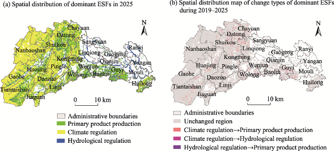
Table 5 The transfer area matrix of the dominant ESFs of the ecological space in Qionglai during 2019-2025
TYPE PPP CR HR The area in 2025
PPP (ha) 29937 2323 533 32793
CR (ha) 0 52490 0 52490
HR (ha) 0 47 12977 13024
The area in 2019 (ha) 29937 54860 13510 98307

Note: PPP, CR, HR have the meanings stated above.

Fig. 6 Spatial distribution maps of the dominant ESFs of Qionglai in 2025 (a) and the change types of dominant ESFs during 2019-2025 (b)
There are two obvious transfer types of dominant ESFs during 2019-2025: “climate regulation → primary product production” and “hydrological regulation → primary product production” (Table 5). Of these two, “climate regulation → primary product production” is the main transfer type of climate regulation function and it transfers out 2370 ha, accounting for 80.02% of the total transfer area of the dominant ESFs in the ecological space, which continues the transfer trend during 2003-2019 (mainly converted to primary product production). Meanwhile, “hydrological regulation → primary product production” is the main transfer type of the hydrological regulation function, and it transfers out 533 ha, accounting for 18.36% of the total transfer area of the dominant ESFs in the ecological space. It shows a trend of increasing transfer area year by year, compared with the transfer area of 2003‒2019.
In the future, there will still be different degrees of conversion between the dominant ESFs of the ecological space in Qionglai City (Fig. 6b). Among them, “climate regulation → primary product production” is mainly distributed in the towns of the western valley region, such as Tiantaishan, Huojing, Datong, Shuikou, Linqiong, etc., and partly distributed in the central and southern parts of the regions with the widest distribution range and the largest change area. The change type of “hydrological regulation → primary product production” is concentrated in Wolong, Baolin and Guyi in the central south, and others are widely scattered in Shuikou and Datong in the northwest with a narrow distribution range and a small change area. It is quite possible, and in line with the strategic regional development plan, for some hydrological regulation functional areas to be transformed into primary product production functional areas in the future, because the central and southern parts of Qionglai City will be planned as an agricultural park to implement the construction of high-standard farmland, according to the Guidelines for the Application of Construction Projects of Qionglai City's Municipal Finance Modern Agricultural Industrial Functional Zone (Park) in 2019.

4 Discussion

4.1 Beneficial contributions of this study

This study addresses three problems related to current research on ecological space: ecological space identification ignores the spatial-temporal dynamics of ecological space brought about by functional evolution, the analysis of ecological space change ignores the influence of dynamics of the dominant ESFs on the future ecological space function pattern, and the composite model integrating the quantitative structure and spatial pattern are applied only rarely to the simulation of the dominant ESFs change in the ecological space. Our study is beneficial because it can complement the eco-spatial planning and management in China and other similar areas, such as the ecological conservation redline delimitation, ecological function regionalization and the construction of the ecological spatial protection pattern.
First, current theoretical research and practical applications for delimiting ecological space (ecological conservation redline) identify the corresponding ranges according to the status assessment results of the regional ecosystem service functions (ecological environmental sensitivity), whereas few consider the spatial-temporal evolutionary characteristics of the ESFs. However, the results of this study confirm that the spatial-temporal dynamic characteristics of ESFs are obvious. Therefore, it is inappropriate to delimit ecological space (ecological conservation redline) based on the ESF status. Hence, in this study, we established a new method for delimiting the ecological space by integrating the dynamics of ESFs during the process of the ecological space demarcation, which we employed to delimit the ecological space for Qionglai City of Sichuan Province, China. The range of the delimited ecological space is consistent with the range of the corresponding ecological function area in the Construction Planning of Ecological Civilization for Qionglai City during 2017-2025. This means that the method for delimiting the ecological space based on the dynamics of ecosystem service functions is relatively reliable, and so this study has partially made up for the deficiencies of the current research and application.
Second, The Planning for National Ecological Function Zoning document and most of the related research delimit the ecological function zones on the basis of the evaluation of ESFs and ecological environmental sensitivity, as well as synthetically integrating the dominant ESFs, regional topography and land use. However, few planning and research efforts consider the dynamic change characteristics of the dominant ESFs during the process of delimiting the ecological function zones, and the results would inevitably experience deviations during the process of guiding the practice of ecological protection and construction as a result of neglecting the future ecological function pattern as it would be influenced by the changes of the dominant ESFs. To address that problem, this study applied the Markov model to analyze the dynamic change characteristics of the dominant ESFs in Qionglai City. The results confirm that the regional dominant ESFs are unstable, i.e., they change over time, and show obvious dynamics. Therefore, during the process of the research and application of ecological function zoning and ecological space zoning management, we should fully consider the dynamics of the dominant ESFs and guide related practices in the future, including ecological space zoning management, ecological function zoning and so on, based on the predicted results for the evolutionary trend of the dominant ESFs.
Third, in order to provide a more scientific and reasonable basis for the related planning, such as ecological function zoning in a given period in the future, simulating the dominant ESFs is of great theoretical and practical significance. However, while a few studies have simulated the dominant ESFs, the spatial simulation models have been applied only rarely to this simulation. In this study, based on the spatial-temporal change characteristics of the dominant ESFs, we tried to simulate the trend of the spatial-temporal changes of the dominant ESFs for the ecological space of Qionglai City in 2025 with the mature spatial change simulation model (Markov-CA), and this process has produced good results. The simulation shows that the ecological space of Qionglai City will have three major ESFs in the future: Primary product production, climate regulation, and hydrological regulation. The spatial pattern of these three functional areas is consistent with the layout of the corresponding ecological function area in the Ecological Function Zoning Map for Qionglai City during 2017-2025. Therefore, it is feasible to employ the Markov-CA model to simulate the trends of changes in the dominant ESFs, and the simulation results were reasonable. On the one hand, this study expanded the application field of spatial simulation models, and enriched the simulation methods of spatial-temporal changes in the dominant ESFs, and also provided a methodological reference for implementing similar research and applications. On the other hand, the results of this study may provide a valuable theoretical support and reference for conducting regional national territory spatial planning and related special planning in the present or future.

4.2 Limitations and improvements of the study

Although, our study solves some problems associated with the current ecological space identification and simulation, there are still some limitations and deficiencies. On the one hand, the time interval of the first period was 2 years shorter than those of the second and third periods during the process of analyzing the characteristics of spatial-temporal changes in the dominant ESFs, because the land use data in 2001 could not be obtained by interpretation due to the poor quality of the remote sensing images. In the future, we could conduct the study with equal intervals by using other methods to obtain land use data with a longer time span. On the other hand, when performing the simulation of the dominant ESF changes, we directly set the map of transfer conditional probabilities of the dominant ESFs as the space transformation rule of CA by the Markov model, referring to related research approaches (Sang et al., 2011; Yang et al., 2012; Yang et al., 2014). Although the simulation precision of this model is high and the simulation method is simple and easy to employ, the depth of the research could be strengthened. In further research we can try to formulate CA model spatial transformation rules based on the evaluation results of the ESFs to simulate the spatial-temporal changes in the dominant ESFs.

5 Conclusions

This paper aims to identify ecological space scientifically and to find a suitable method to simulate the spatial-temporal changes in the dominant ESFs in the ecological space. This paper proposes an ecological space identification method based on the dynamic change characteristics of the ESFs, realizing the successful identification of ecological space in Qionglai City. On this basis, this paper also integrates a Markov-CA model with the spatial-temporal change characteristics of the dominant ESFs, successfully predicting the spatial pattern of the dominant ESFs in Qionglai City in 2025, revealing a suitable method for the simulation of ecological spatial change and providing a basic support for constructing reasonable ecological space protection patterns.
At present, there are some obvious deficiencies in the research of ecological space identification and simulation. Firstly, the ecological space identification is mainly based on the information of the current ecosystem structure and function, but ignores the spatial-temporal dynamics of ecological space brought by functional evolution. Secondly, the analysis of ecological spatial evolution ignores the influence of the dominant ESF dynamics on the future ecological spatial function pattern. Thirdly, the simulation of future ESF changes in ecological space is not emphasized. In particular, the composite model coupled with quantitative structure and spatial layout is rarely applied in the simulation of the dominant ESF changes, failing to provide a good technical and methodological support for constructing the ecological spatial protection pattern.
The proposed methods of delimiting ecological space and simulating spatial-temporal changes in the dominant ESFs from the perspective of the ESF dynamic changes solve the above problems, and the feasibility of these methods was proven by the ecological spatial identification and the simulation of the dominant ESFs of Qionglai. The results confirm that: 1) The comprehensive ESF quantity and its inter-annual change rate in Qionglai City showed obvious dynamics, so it is necessary to consider the dynamic characteristics of the ESFs when identifying ecological space. 2) The critical values of its comprehensive function quantity and its change rate for dividing ecological space and non-ecological space are 6.79 and 5%, respectively. The ecological space area of Qionglai City is 98307 ha, accounting for 71.39% of the total territorial space area, which is mainly concentrated in the west and central south. This is basically consistent with the corresponding ecological spatial distribution determined in the local ecological civilization construction plans, proving that the method based on the dynamic characteristics of ESFs is reliable. 3) The dominant ESFs of the ecological space in Qionglai City have shifted to varying degrees, showing strong dynamics during 2003-2019 and 2019-2025, further confirming the non- stationary nature of the dominant ESFs. So, we should fully consider the influence of the dynamics in the dominant ESFs on the future ecological space pattern in the construction of the ecological space protection pattern. 4) The Markov-CA model accurately simulated the spatial-temporal changes in the dominant ESFs in Qionglai City, with a Kappa coefficient above 0.95, indicating that it is feasible to use this model to simulate the spatial pattern of the dominant ESFs in the future. The simulation results show that the dominant ESFs in Qionglai city will still undergo mutual conversions due to the instability of the ESFs. The ecological space will still maintain three dominant functions in 2025, including primary product production, climate regulation and hydrological regulation, but their areas will change to 32793 ha, 52490 ha and 13024 ha, respectively.
In conclusion, there are three main beneficial results from our research. Firstly, we propose an ecological space identification method based on the dynamics of the ESFs, which enhances the rationality and reliability of ecological space delimitation. Secondly, this study further confirms the non-stationary nature of the dominant ESFs, and provides a theoretical basis for considering the influence of the dynamics of the dominant ESFs on the future ecological space function pattern, and for the necessary simulation of the spatial-temporal changes of the dominant ESFs when constructing the ecological space protection pattern. Thirdly, we successfully applied the Markov-CA model to the simulation of spatial-temporal changes in the dominant ESFs, confirming that it is a suitable method for the simulation of spatial-temporal changes in the dominant ESFs in ecological space, and providing a basic support for the construction of the ecological space protection pattern.
[1]
Al-Ahmadi K, See L D, Heppenstall A, et al. 2009. Calibration of a fuzzy cellular automata model of urban dynamics in Saudi Arabia. Ecological Complexity, 6(2): 80-101.

DOI

[2]
Al-sharif A A A, Pradhan B. 2014. Monitoring and predicting land use change in Tripoli Metropolitan City using an integrated Markov chain and cellular automata models in GIS. Arabian Journal of Geosciences, 7(10): 4291-4301.

DOI

[3]
Chen Y, Yue W Z, Zhang L, et al. 2020. Theoretical thinking on ecological space zoning from the perspective of territorial space planning. China Land Science, 34(8): 1-9. (in Chinese?)

[4]
Cicchetti D V, Feinstein A R. 1990. High agreement but low Kappa: II. Resolving the paradoxes. Journal of Clinical Epidemiology, 43(6): 551-558.

PMID

[5]
Costanza R, d'Arge R, de Groot R, et al. 1997. The value of the world's ecosystem services and natural capital. Nature, 387(6630): 253-260.

DOI

[6]
Costanza R, de Groot R, Sutton P, et al. 2014. Changes in the global value of ecosystem services. Global Environmental Change, 26(1): 152-158.

DOI

[7]
Daily G C. 1999. Developing a scientific basis for managing earth's life support systems. Ecology & Society, 3(2): 45-49.

[8]
Daily G C, Soderqvist T, Aniyar S, et al. 2000. The value of nature and the nature of value. Science, 289(5478): 395-396.

[9]
Feinstein A R, Cicchetti D V. 1990. High agreement but low Kappa: I. The problems of two paradoxes. Journal of Clinical Epidemiology, 43(6): 543-549.

DOI PMID

[10]
Feng Y J, Liu Y, Tong X H, et al. 2011. Modeling dynamic urban growth using cellular automata and particle swarm optimization rules. Landscape and Urban Planning, 102(3): 188-196.

DOI

[11]
Gao J, Yu Z W, Wang L C, et al. 2019. Suitability of regional development based on ecosystem service benefits and losses: A case study of the Yangtze River Delta urban agglomeration, China. Ecological Indicators, 107: 105579. 1-105579.12.

[12]
Gao J X, Xu D L, Qiao Q, et al. 2020. Pattern construction of natural ecological space and planning theory exploration. Acta Ecologica Sinica, 40(3): 749-755. (in Chinese)

[13]
Guan X K, Zhang F R, Wang X L, et al. 2013. Spatial evolution of urban ecological land and its distribution optimization in Beijing. Areal Research and Development, 32(3): 119-124. (in Chinese)

[14]
Halmy M W A, Gessler P E, Hicke J A, et al. 2015. Land use/land cover change detection and prediction in the north-western coastal desert of Egypt using Markov-CA. Applied Geography, 63: 101-112.

DOI

[15]
Kucsicsa G, Popovici E.A, Bălteanu D, et al. 2019. Future land use/cover changes in Romania: Regional simulations based on CLUE-S model and CORINE land cover database. Landscape and Ecological Engineering, 15(1): 75-90.

[16]
Kumar P, Rosenberger J M, Iqbal G M D. 2016. Mixed integer linear programming approaches for land use planning that limit urban sprawl. Computers & Industrial Engineering, 102: 33-43.

DOI

[17]
Li M Y, Tian F H, Dong Y Z. 2016. Space identification of ecological importance and protection on urban ecological land in Yanji-Longjing-Tumen Area. Scientia Geographical Sinica, 36(12): 1870-1876. (in Chinese)

[18]
Ma C G, Zhou M. 2018. A GIS-based interval fuzzy linear programming for optimal land resource allocation at a city scale. Social Indicators Research, 135(1): 143-166.

DOI

[19]
Moreno N, Menard A, Marceau D J. 2008. VecGCA: A vector-based geographic cellular automata model allowing geometric transformations of objects. Environment & Planning B: Planning & Design, 35(4): 647-665.

[20]
Pahlavani P, Omaran H A, Bigdeli B. 2017. A multiple land use change model based on artificial neural network, Markov chain, and multi objective land allocation. Earth Observation and Geomatics Engineering, 1(2): 82-99.

[21]
Sang L L, Zhang C, Yang J Y, et al. 2011. Simulation of land use spatial pattern of towns and villages based on CA-Markov model. Mathematical and Computer Modelling, 54(3-4): 938-943.

DOI

[22]
Shi Y, Wang R S, Huang J L, et al. 2012. An analysis of the spatial and temporal changes in Chinese terrestrial ecosystem service functions. Chinese Science Bulletin, 57(17): 2120-2131.

DOI

[23]
Wang S D, Wang X C, Zhang H B. 2015. Simulation on optimized allocation of land resource based on DE-CA model. Ecological Modelling, 314: 135-144.

DOI

[24]
Wang W J, Guo H C, Chuai X W, et al. 2014. The impact of land use change on the temporospatial variations of ecosystems services value in China and an optimized land use solution. Environmental Science & Policy, 44: 62-72.

[25]
Wang X, Ma B W, Li D, et al. 2020. Multi-scenario simulation and prediction of ecological space in Hubei Province based on FLUS model. Journal of Natural Resources, 35(1): 230-242. (in Chinese)

DOI

[26]
Xie G D, Lu C X, Leng Y F, et al. 2003. Value evaluation of ecological assets of Qinghai-Tibet Plateau. Journal of Natural Resources, 18(2): 189-196. (in Chinese)

[27]
Xie G D, Zhang C X, Zhang L M, et al. 2015. Improvement of the evaluation method for ecosystem service value based on per unit area. Journal of Natural Resources, 30(8): 1243-1254. (in Chinese)

[28]
Xie G D, Zhen L, Lu C X, et al. 2008. A method of ecosystem services based on expert knowledge. Natural Resources, 23(5): 911-919. (in Chinese)

[29]
Xie G D, Zhen L, Lu C X, et al. 2010. Applying value transfer method for Eco-service valuation in China. Journal of Resources and Ecology, 1(1): 51-59.

[30]
Xie H L, Yao G, He Y F, et al. 2018. Study on spatial identification of critical ecological space based on GIS: A case study of Poyang Lake Ecological Economic Zone. Acta Ecologica Sinica, 38(16): 5926-5937. (in Chinese)

[31]
Xu H L, Gao W L, Chen S, et al. 2020. Identification of urban ecological space in South Jiangsu based on GIS: A case study of Suzhou. Chinese. Journal of Ecology, 39(2): 614-624. (in Chinese)

[32]
Yang X, Zheng X Q, Chen R. 2014. A land use change model: Integrating landscape pattern indexes and Markov-CA. Ecological Modelling, 283: 1-7.

DOI

[33]
Yang X, Zheng X Q, Lv L N. 2012. A spatiotemporal model of land use change based on ant colony optimization, Markov chain and cellular automata. Ecological Modelling, 233: 11-19.

DOI

[34]
Yao N, Ma L Y, Yang J, et al. 2015. Changes of ecological spaces in Beijing's Plain areas between 1992 and 2013. Chinese Journal of Ecology, 34(5): 1427-1434. (in Chinese)

[35]
Zhang Y P, Chang Q, Guo X D. 2016. Management-oriented ecological land's conception and multi-dimensional classification system in China. Acta Ecologica Sinica, 36(12): 3655-3665. (in Chinese)

[36]
Zhao T Q, Ouyang Z Y, Jia L Q, et al. 2004. Ecosystem services and their valuation of China grassland. Acta Ecologica Sinica, 24(6): 1101-1110. (in Chinese)

[37]
Zhou R, Zhang H, Ye X Y, et al. 2016. The delimitation of urban growth boundaries using the CLUE-S land-use change model: Study on Xinzhuang Town, Changshu City, China. Sustainability, 8(11): 1182. DOI: 10.3390/su8111182.

DOI

Outlines

/