
Journal of Resources and Ecology >
The Effects of Tourism Industry Agglomeration on Tourism Environmental Carrying Capacity: Evidence from a Panel Threshold Model
Received date: 2021-10-15
Accepted date: 2022-05-30
Online published: 2022-10-12
Supported by
The National Social Science Fund Project of China(21BGL021)
The National Social Science Fund Project of China(19BGL138)
The Macro Decision-making Projects on Culture and Tourism of China Tourism Academy(2021HGJCG04)
The Natural Science Planning Project in Shandong Province(ZR202102200015)
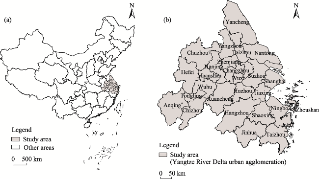
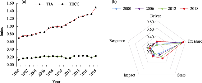
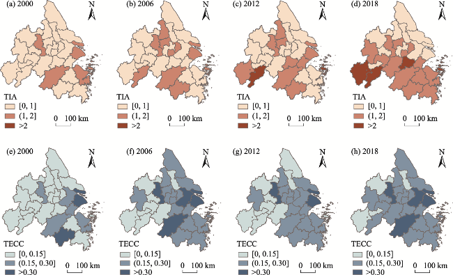
By utilizing the panel data of 26 cities in the Yangtze River Delta urban agglomeration of China from 2000 to 2018, this study constructs a panel threshold model to examine the nonlinear relationship between Tourism Environmental Carrying Capacity (TECC) and Tourism Industry Agglomeration (TIA). TECC is evaluated based on the Driver-Pressure-State-Impact-Response (DPSIR) model, and TIA is estimated by the location quotient index. The analysis reveals that TIA and TECC both show growth trends and significant regional differences among the 26 cities, but the latter fluctuates at certain stages. Moreover, TIA has a significant double threshold effect on TECC, which shows that the positive impact of TIA is enhanced initially but then weakens afterwards. Theoretically, this study contributes to enriching the current literature on TECC from the perspective of TIA. Practically, it could help local governments effectively arrange agglomerations to promote the sustainable development of the tourism industry in China.
LIU Jia , LI Jing , AN Keke . The Effects of Tourism Industry Agglomeration on Tourism Environmental Carrying Capacity: Evidence from a Panel Threshold Model[J]. Journal of Resources and Ecology, 2022 , 13(6) : 1037 -1047 . DOI: 10.5814/j.issn.1674-764x.2022.06.009
Fig. 1 Location of the study area |
Table 1 Evaluation index system of TECC |
| Target | Subsystems | Indicators | Indicator interpretations |
|---|---|---|---|
| TECC | Driver (D) | GDP (D1) | Represents the driving force of economic aggregate on TECC |
| Per capita disposable income of households (D2) | Represents the driving force of economic development level on TECC | ||
| Ratio of the number of tourists to the number of residents (D3) | Represents the driving force of tourist crowding on TECC | ||
| Turnover of passenger traffic (D4) | Represents the driving force of tourist turnover on TECC | ||
| Number of tourists (D5) | Represents the driving force of tourist stay on TECC | ||
| Pressure (P) | Energy consumption per unit of GDP (P1) | Represents the pressure of energy consumption on TECC | |
| Electricity consumption per unit of GDP (P2) | Represents the pressure of electricity consumption on TECC | ||
| Water consumption per unit of GDP (P3) | Represents the pressure of water consumption on TECC | ||
| State (S) | Number of A-grade tourist attractions (S1) | Represents the number of tourism resources | |
| Number of tourist attractions above AAAA-grade (S2) | Represents the quality of tourism resources | ||
| Number of air quality standard days (S3) | Represents the quality of air | ||
| Impact (I) | Total tourism revenue (I1) | Represents the impact of TECC on tourism economy | |
| Tourism earnings as percentage of GDP (I2) | Represents the impact of TECC on industrial structure | ||
| Tertiary industry product as percentage of GDP (I3) | Represents the impact of TECC on economic structures | ||
| Number of tourism professionals (I4) | Represents the impact of TECC on regional employment | ||
| Per capita consumption expenditure of households (I5) | Represents the impact of TECC on residents' consumption expenditure | ||
| Response (R) | Number of cultural and art institutions (R1) | Represents the response of infrastructure to TECC | |
| Ratio of waste water centralized treated of sewage work (R2) | Represents the response of water quality optimization to TECC | ||
| Ratio of consumption on wastes treated (R3) | Represents the response of waste utilization to TECC | ||
| Green covered area as percentage of built-up area (R4) | Represents the response of air quality optimization to TECC | ||
| Investment in anti-pollution projects as percentage of GDP (R5) | Represents the response of government governance to TECC | ||
| Actual utilization of foreign capital as percentage of GDP (R6) | Represents the response of regional openness to TECC | ||
| Intramural expenditure on R&D as percentage of GDP (R7) | Represents the response of scientific research investment to TECC | ||
| Number of taxis (R8) | Represents the response of infrastructure to TECC | ||
| Number of hospitals (R9) | Represents the response of public services to TECC | ||
| Per capita years of school attainment (R10) | Represents the response of tourism residents to TECC | ||
| Number of students enrolled in regular institutions of higher education (R11) | Represents the response of practitioner quality to TECC |
Table 2 Definitions of variables |
| Variables | Attributes | Measurements |
|---|---|---|
| Tourism environmental carrying capacity (TECC) | Dependent variable | Entropy weight method |
| Tourism industry agglomeration (TIA) | Independent variable | Location quotient |
| Economic development level (ECO) | Control variable | Per capita disposable income |
| Tourist density (DEN) | Control variable | Ratio of the number of tourists to the number of residents |
| Tourism ecological efficiency (EFF) | Control variable | Super-efficiency SBM model |
| Technological progress level (TEC) | Control variable | Science and technology expenditure/local government financial expenditure |
| Environmental regulation strength (ERS) | Control variable | Investment in anti-pollution projects as percentage of GDP |
Table 3 Matrix of correlations |
| Variables | TIA | ECO | DEN | EFF | TEC | ERS |
|---|---|---|---|---|---|---|
| TIA | 1.0000 | |||||
| ECO | 0.2431 | 1.0000 | ||||
| DEN | 0.0029 | 0.0140 | 1.0000 | |||
| EFF | 0.5018 | 0.6258 | -0.0095 | 1.0000 | ||
| TEC | 0.0288 | 0.6843 | 0.0225 | 0.3638 | 1.0000 | |
| ERS | 0.1151 | 0.0737 | 0.0024 | 0.2215 | 0.0099 | 1.0000 |
Fig. 2 The temporal evolution of the TIA and TECC (a) and the five subsystems (b) |
Fig. 3 The spatial evolution of the TIA (a-d) and TECC (e-h) |
Table 4 Test of the threshold effect |
| Type of threshold test | 95% confidence interval | F-statistic | P-value | Threshold estimate | Critical value | ||
|---|---|---|---|---|---|---|---|
| 1% | 5% | 10% | |||||
| Single threshold model | [1.194, 1.217] | 19.832** | 0.022 | 1.217 | 21.426 | 17.807 | 15.074 |
| Double threshold model | [0.974, 2.460]; [0.931, 1.064] | 57.151*** | 0.000 | 0.991; 1.626 | -12.300 | -18.261 | -21.545 |
Note: ** and *** indicate the tests are significant at levels of 5% and 1%, respectively. The triple threshold test is not significant, so the results are not listed here. |
Table 5 Numbers and proportions of the 26 sample cities in the two threshold value intervals |
| Year | Across the first threshold 0.991 | First threshold crossing rate (%) | Across the second threshold 1.626 | Second threshold crossing rate (%) |
|---|---|---|---|---|
| 2000 | 5 | 19.23 | 1 | 3.85 |
| 2001 | 4 | 15.39 | 0 | 0 |
| 2002 | 4 | 15.39 | 0 | 0 |
| 2003 | 5 | 19.23 | 1 | 3.85 |
| 2004 | 5 | 19.23 | 1 | 3.85 |
| 2005 | 7 | 26.92 | 1 | 3.85 |
| 2006 | 9 | 34.62 | 1 | 3.85 |
| 2007 | 10 | 38.46 | 2 | 7.69 |
| 2008 | 8 | 30.77 | 2 | 7.69 |
| 2009 | 10 | 38.46 | 2 | 7.69 |
| 2010 | 10 | 38.46 | 2 | 7.69 |
| 2011 | 9 | 34.62 | 2 | 7.69 |
| 2012 | 11 | 42.31 | 2 | 7.69 |
| 2013 | 15 | 57.69 | 2 | 7.69 |
| 2014 | 15 | 57.69 | 3 | 11.54 |
| 2015 | 15 | 57.69 | 4 | 15.39 |
| 2016 | 15 | 57.69 | 4 | 15.39 |
| 2017 | 14 | 53.85 | 5 | 19.23 |
| 2018 | 16 | 61.54 | 5 | 19.23 |
Table 6 Test results of the double threshold of TIA |
| Variable | Regression coefficient | T-statistic | P value |
|---|---|---|---|
| ECO | 0.001* | 1.80 | 0.072 |
| DEN | 0.001*** | 6.73 | 0.000 |
| ERS | 1.373*** | 4.84 | 0.000 |
| TEC | 0.466*** | 3.75 | 0.000 |
| EFF | 0.024** | 2.10 | 0.036 |
| TIA≤0.991 | 0.028*** | 2.58 | 0.010 |
| 0.991<TIA≤1.626 | 0.053*** | 6.85 | 0.000 |
| TIA>1.626 | 0.023*** | 5.72 | 0.000 |
Note: *, **, and *** indicate the tests are significant at levels of 10%, 5%, and 1%, respectively. |
| [1] |
|
| [2] |
|
| [3] |
|
| [4] |
|
| [5] |
|
| [6] |
|
| [7] |
|
| [8] |
|
| [9] |
|
| [10] |
|
| [11] |
|
| [12] |
|
| [13] |
|
| [14] |
|
| [15] |
|
| [16] |
|
| [17] |
|
| [18] |
|
| [19] |
|
| [20] |
|
| [21] |
|
| [22] |
|
| [23] |
|
| [24] |
|
| [25] |
|
| [26] |
|
| [27] |
|
| [28] |
|
| [29] |
|
| [30] |
|
| [31] |
|
| [32] |
|
| [33] |
|
| [34] |
|
| [35] |
|
| [36] |
|
| [37] |
|
| [38] |
|
| [39] |
|
| [40] |
|
| [41] |
|
| [42] |
|
| [43] |
|
| [44] |
|
| [45] |
|
| [46] |
|
| [47] |
|
| [48] |
|
| [49] |
|
| [50] |
|
| [51] |
|
| [52] |
|
| [53] |
|
| [54] |
|
| [55] |
|
| [56] |
|
| [57] |
|
| [58] |
|
| [59] |
|
| [60] |
|
| [61] |
|
/
| 〈 |
|
〉 |