
Journal of Resources and Ecology >
Spatio-temporal Evolution and Flow of Water Provision Service Balance in Jinghe River Basin
|
GUAN Mengluan, E-mail: guanml@craes.org.cn |
Received date: 2021-11-01
Accepted date: 2022-04-20
Online published: 2022-07-15
Supported by
The National Natural Science Foundation of China(41701601)
The National Natural Science Foundation of China(41871196)
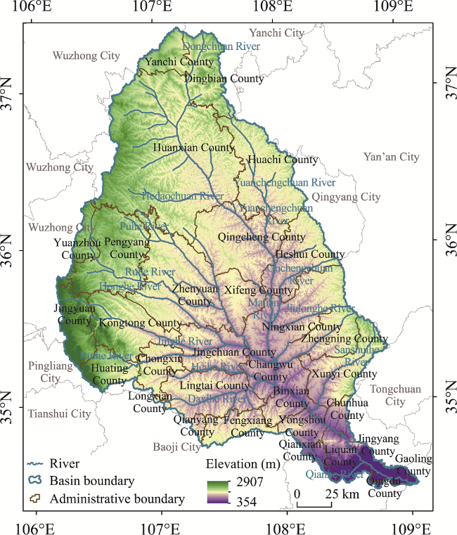
Quantifying the whole process of ecosystem services from generation through transfer to use, and analyzing the balance between the supply and demand of regional ecosystem services are of great significance for formulating regional sustainable development strategies, realizing regional ecosystem management, and effective resource allocation. Based on the SWAT model, InVEST model, ArcGIS, and other software, this study analyzed the supply-demand balance of water provision services in Jinghe River Basin, a typical region located in the Loess Plateau, using multi-source data. This research then analyzed the spatial-temporal distribution pattern and spatial matching characteristics of the supply and demand of water provision services in Jinghe River Basin from 2000 to 2015. On this basis, a spatial flow model of water provision service was constructed, the flow rules (flow paths) of the water provision service were explored at the subwatershed scale, and the spatial scope of the supply area and benefit area were depicted. The results show that: (1) Water resource supply and demand in the Jinghe River basin both showed increasing trends from 2000 to 2015. (2) The supply-demand balance of water resources was generally up to the standard, however, there were significant differences between urban and rural areas. The supply-demand balances of the central urban areas of each county were relatively low, and even exceeded the supply in the lower reaches of the Jingyang River, such as Gaoling County, Qindu District, and Jingyang County. In rural areas, due to the small population and industrial distribution, coupled with a better ecological environmental base, the supply-demand balance was relatively high, such as Pengyang County, Lingtai County, Huachi County, Huanxian County, Ningxian County, and Zhenyuan County. (3) From 2000 to 2015, the spatial matching pattern of supply and demand in the Jinghe River Basin showed a trend of decline with fluctuations. In 2015, the supply-demand ratios of more than 60% of the subwatersheds showed trends of decline, and the proportion of under-supply area increased by 55.7% in 2015 compared with that in 2000. (4) The supply areas of water provision service in Jinghe River Basin are distributed in the upper reaches of the basin, and the benefit areas are Huating County, Chongxin County, Yongshou County, Chunhua County, Ganxian County, Liquan County, Qindu District, and others in the middle and lower reaches.
GUAN Mengluan , ZHANG Qiang , WANG Baoliang , ZHANG Huiyuan . Spatio-temporal Evolution and Flow of Water Provision Service Balance in Jinghe River Basin[J]. Journal of Resources and Ecology, 2022 , 13(5) : 797 -812 . DOI: 10.5814/j.issn.1674-764x.2022.05.005
Fig. 1 Location of the study area and the distribution of the rivers, digital elevation model (DEM), and administrative boundaries. |
Table 1 Maximum root depths and evapotranspiration coefficients of the different land use types |
| Code | Land use type | Maximum root depth (mm) | Evapotranspiration coefficient |
|---|---|---|---|
| 1 | Woodland | 4000 | 1 |
| 2 | Grassland | 500 | 0.65 |
| 3 | Wetland | 300 | 1.2 |
| 4 | Arable land | 300 | 0.65 |
| 5 | Artificial surface | 1 | 0.3 |
| 6 | Other | 1 | 0.3 |
Table 2 Per capita water consumption in Jinghe River Basin from 2000 to 2015 (Unit: m3 person-1) |
| Year | 2000 | 2005 | 2010 | 2015 |
|---|---|---|---|---|
| Per capita water consumption | 865.35 | 1314.2 | 1162.35 | 1053.65 |
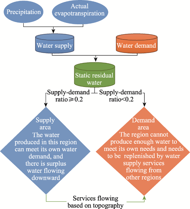
Fig. 2 Schematic diagram of the water provision service spatial flow model in Jinghe River Basin |
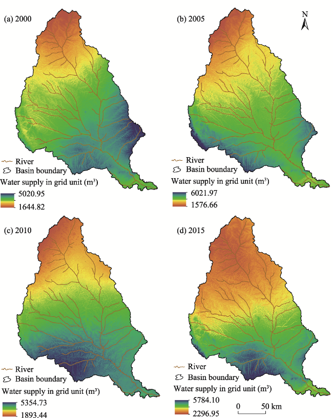
Fig. 3 Spatial distribution of the water supply in grid unit in Jinghe River Basin from 2000 to 2015 |
Table 3 Average water conservation depth and water supply amount in Jinghe River Basin during 2000-2015 |
| Year | Depth of water conservation (mm) | Water supply (108 m3) |
|---|---|---|
| 2000 | 424.03 | 187.47 |
| 2005 | 397.59 | 175.78 |
| 2010 | 479.49 | 211.99 |
| 2015 | 458.39 | 202.66 |
Table 4 Water supply by counties (districts) in Jinghe River Basin from 2000 to 2015 (Unit: 108 m3) |
| City | County | 2000 | 2005 | 2010 | 2015 | City | County | 2000 | 2005 | 2010 | 2015 |
|---|---|---|---|---|---|---|---|---|---|---|---|
| Baoji | Fengxiang | 4.45 | 4.29 | 5.10 | 5.43 | Qingyang | Xifeng | 4.70 | 4.14 | 5.19 | 4.86 |
| Longxian | 0.25 | 0.28 | 0.33 | 0.31 | Zhenyuan | 14.68 | 13.65 | 17.53 | 15.53 | ||
| Qianyang | 0.73 | 0.76 | 0.90 | 0.91 | Zhengning | 7.21 | 6.26 | 7.16 | 7.21 | ||
| Guyuan | Pengyang | 9.91 | 9.27 | 11.36 | 10.14 | Wuzhong | Yanchi | 1.81 | 1.77 | 2.18 | 2.60 |
| Yuanzhou | 2.05 | 1.85 | 2.23 | 2.01 | Xi’an | Gaoling | 0.22 | 0.21 | 0.27 | 0.25 | |
| Jingyuan | 4.62 | 5.39 | 5.73 | 5.69 | Xianyang | Binxian | 6.03 | 5.32 | 6.82 | 6.82 | |
| Pingliang | Chongxin | 3.82 | 4.09 | 5.04 | 4.65 | Changwu | 2.84 | 2.48 | 3.29 | 3.22 | |
| Huating | 3.71 | 4.61 | 5.14 | 4.81 | Chunhua | 1.93 | 1.74 | 2.13 | 2.17 | ||
| Lingtai | 9.94 | 9.53 | 11.99 | 11.99 | Liquan | 3.58 | 3.29 | 4.27 | 4.15 | ||
| Kongtong | 7.96 | 8.45 | 10.46 | 9.40 | Qianxian | 0.96 | 0.90 | 1.15 | 1.14 | ||
| Jingchuan | 7.10 | 6.48 | 8.51 | 8.13 | Qindu | 0.23 | 0.21 | 0.27 | 0.26 | ||
| Qingyang | Heshui | 8.64 | 7.37 | 8.57 | 8.01 | Xunyi | 9.11 | 8.08 | 9.12 | 9.45 | |
| Huachi | 10.26 | 9.35 | 10.11 | 9.77 | Yongshou | 3.13 | 2.84 | 3.55 | 3.66 | ||
| Huanxian | 26.93 | 25.61 | 30.18 | 28.35 | Jingyang | 2.16 | 1.98 | 2.63 | 2.44 | ||
| Ningxian | 13.45 | 11.53 | 14.07 | 13.42 | Yulin | Dingbian | 3.57 | 3.79 | 4.42 | 4.80 | |
| Qingcheng | 11.51 | 10.28 | 12.34 | 11.12 |
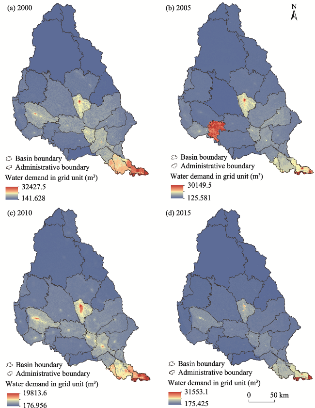
Fig. 4 Temporal and spatial distribution of water resource demand of the individual grid unit in the Jinghe River Basin from 2000 to 2015 |
Table 5 Water demand of counties (districts) in Jinghe River Basin from 2000 to 2015 (Unit: 108 m3) |
| City | County | 2000 | 2005 | 2010 | 2015 |
|---|---|---|---|---|---|
| Baoji | Fengxiang | 0.41 | 0.66 | 0.58 | 0.54 |
| Longxian | 0.05 | 0.11 | 0.07 | 0.06 | |
| Qianyang | 0.14 | 0.22 | 0.18 | 0.18 | |
| Guyuan | Pengyang | 1.97 | 2.85 | 2.37 | 2.10 |
| Yuanzhou | 0.56 | 1.00 | 0.67 | 0.63 | |
| Jingyuan | 1.09 | 2.24 | 1.17 | 1.06 | |
| Pingliang | Chongxin | 0.87 | 11.80 | 1.22 | 1.13 |
| Huating | 1.10 | 3.11 | 1.68 | 1.54 | |
| Lingtai | 1.80 | 2.62 | 2.05 | 1.86 | |
| Kongtong | 3.90 | 2.42 | 5.87 | 5.48 | |
| Jingchuan | 2.59 | 2.31 | 3.25 | 2.98 | |
| Qingyang | Heshui | 0.86 | 1.99 | 1.15 | 1.05 |
| Huachi | 0.78 | 1.76 | 1.02 | 0.95 | |
| Huanxian | 2.53 | 3.05 | 3.26 | 2.99 | |
| Ningxian | 4.20 | 6.64 | 4.89 | 4.42 | |
| Qingcheng | 2.72 | 3.46 | 3.05 | 2.80 | |
| Xifeng | 2.76 | 6.57 | 4.36 | 3.99 | |
| Zhenyuan | 4.24 | 0.95 | 4.84 | 4.44 | |
| Zhengning | 1.80 | 4.73 | 2.26 | 2.08 | |
| Wuzhong | Yanchi | 0.19 | 0.35 | 0.24 | 0.23 |
| Xi’an | Gaoling | 0.33 | 0.72 | 0.72 | 1.10 |
| Xianyang | Binxian | 2.65 | 4.19 | 3.66 | 3.35 |
| Changwu | 1.45 | 2.29 | 1.83 | 1.69 | |
| Chunhua | 0.65 | 1.08 | 0.91 | 0.85 | |
| Liquan | 2.89 | 4.48 | 3.90 | 3.64 | |
| Qianxian | 0.84 | 1.43 | 1.22 | 1.12 | |
| Qindu | 0.68 | 1.00 | 0.93 | 0.94 | |
| Xunyi | 2.16 | 3.46 | 2.82 | 2.60 | |
| Yongshou | 1.35 | 1.92 | 1.56 | 1.45 | |
| Jingyang | 2.55 | 4.16 | 3.69 | 3.41 | |
| Yulin | Dingbian | 0.52 | 0.88 | 0.85 | 0.73 |
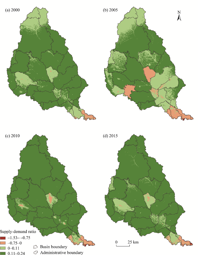
Fig. 5 Temporal and spatial distribution of the water provision service supply-demand ratios in Jinghe River Basin from 2000 to 2015Note: Negative values indicate demand exceed supply. |
Table 6 Supply-demand ratios of water provision services among the counties (districts) in Jinghe River Basin from 2000 to 2015 |
| City | County | 2000 | 2005 | 2010 | 2015 |
|---|---|---|---|---|---|
| Baoji | Fengxiang | 0.26 | 0.19 | 0.25 | 0.29 |
| Longxian | 0.01 | 0.01 | 0.01 | 0.02 | |
| Qianyang | 0.04 | 0.03 | 0.04 | 0.04 | |
| Guyuan | Pengyang | 0.51 | 0.34 | 0.50 | 0.48 |
| Yuanzhou | 0.10 | 0.05 | 0.09 | 0.08 | |
| Jingyuan | 0.23 | 0.17 | 0.25 | 0.27 | |
| Pingliang | Chongxin | 0.19 | -0.41 | 0.21 | 0.21 |
| Huating | 0.17 | 0.08 | 0.19 | 0.19 | |
| Lingtai | 0.52 | 0.37 | 0.55 | 0.60 | |
| Kongtong | 0.26 | 0.32 | 0.25 | 0.23 | |
| Jingchuan | 0.29 | 0.22 | 0.29 | 0.31 | |
| Qingyang | Heshui | 0.50 | 0.29 | 0.41 | 0.41 |
| Huachi | 0.61 | 0.41 | 0.50 | 0.52 | |
| Huanxian | 1.57 | 1.21 | 1.49 | 1.50 | |
| Ningxian | 0.59 | 0.26 | 0.51 | 0.53 | |
| Qingcheng | 0.57 | 0.37 | 0.52 | 0.49 | |
| Xifeng | 0.13 | -0.13 | 0.05 | 0.05 | |
| Zhenyuan | 0.67 | 0.68 | 0.70 | 0.66 | |
| Zhengning | 0.35 | 0.08 | 0.27 | 0.30 | |
| Wuzhong | Yanchi | 0.10 | 0.08 | 0.11 | 0.14 |
| Xi’an | Gaoling | -0.01 | -0.03 | -0.03 | -0.05 |
| Xianyang | Binxian | 0.22 | 0.06 | 0.18 | 0.21 |
| Changwu | 0.09 | 0.01 | 0.08 | 0.09 | |
| Chunhua | 0.08 | 0.04 | 0.07 | 0.08 | |
| Liquan | 0.04 | -0.06 | 0.02 | 0.03 | |
| Qianxian | 0.01 | -0.03 | 0.00 | 0.00 | |
| Qindu | -0.03 | -0.04 | -0.04 | -0.04 | |
| Xunyi | 0.45 | 0.25 | 0.35 | 0.41 | |
| Yongshou | 0.11 | 0.05 | 0.11 | 0.13 | |
| Jingyang | -0.03 | -0.12 | -0.06 | -0.06 | |
| Yulin | Dingbian | 0.20 | 0.16 | 0.20 | 0.24 |
Note: Negative values indicate demand exceed supply. The same below. |
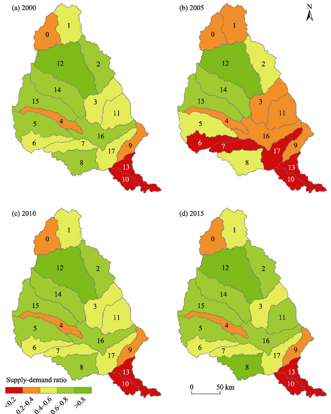
Fig. 6 Spatial and temporal distribution of the supply-demand ratios of water provision services in each subwatershed of the Jinghe River Basin from 2000 to 2015.Note: The numbers 0-17 denote the codes of the subwatersheds in Jinghe River Basin. |
Table 7 Supply-demand ratios of water provision services in each of the subwatersheds of the Jinghe River Basin from 2000 to 2015 |
| Subwatershed number | 2000 | 2005 | 2010 | 2015 |
|---|---|---|---|---|
| 0 | 0.37 | 0.28 | 0.33 | 0.40 |
| 1 | 0.43 | 0.38 | 0.44 | 0.53 |
| 2 | 0.79 | 0.58 | 0.65 | 0.68 |
| 3 | 0.65 | 0.27 | 0.50 | 0.50 |
| 4 | 0.31 | 0.31 | 0.32 | 0.31 |
| 5 | 0.59 | 0.58 | 0.60 | 0.60 |
| 6 | 0.38 | -0.09 | 0.42 | 0.42 |
| 7 | 0.39 | 0.04 | 0.41 | 0.44 |
| 8 | 0.78 | 0.58 | 0.78 | 0.88 |
| 9 | 0.40 | 0.25 | 0.31 | 0.36 |
| 10 | 0.09 | -0.08 | 0.05 | 0.08 |
| 11 | 0.72 | 0.37 | 0.57 | 0.60 |
| 12 | 1.37 | 1.12 | 1.28 | 1.24 |
| 13 | 0.12 | -0.17 | 0.02 | 0.01 |
| 14 | 0.81 | 0.61 | 0.74 | 0.72 |
| 15 | 0.75 | 0.62 | 0.73 | 0.70 |
| 16 | 0.72 | 0.27 | 0.61 | 0.67 |
| 17 | 0.50 | 0.19 | 0.41 | 0.48 |
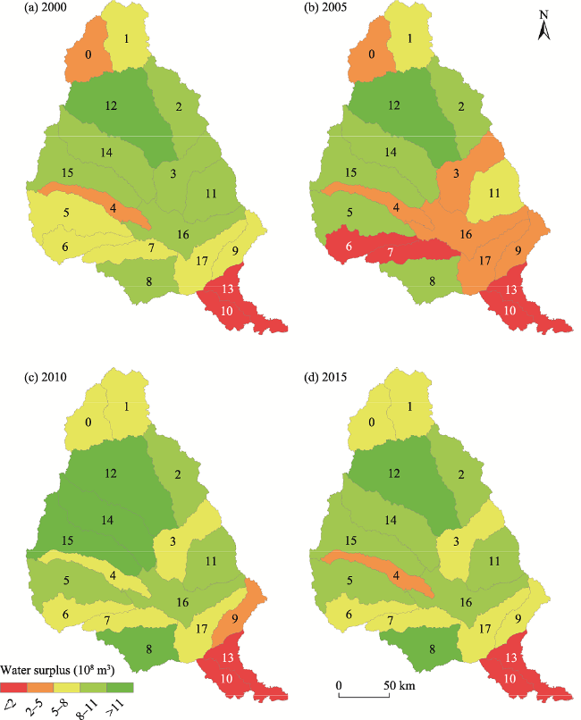
Fig. 7 The surplus water in each subwatershed in the Jinghe River Basin from 2000 to 2015Note: The numbers 0-17 denote the codes of the subwatersheds in Jinghe River Basin. |
Fig. 8 The demand area and supply area at the subwatershed scale in the Jinghe River Basin from 2000 to 2015Note: The numbers 0-17 denote the codes of the subwatersheds in Jinghe River Basin. |
| [1] |
|
| [2] |
|
| [3] |
|
| [4] |
|
| [5] |
|
| [6] |
|
| [7] |
|
| [8] |
|
| [9] |
|
| [10] |
|
| [11] |
|
| [12] |
|
| [13] |
|
| [14] |
|
| [15] |
|
| [16] |
|
| [17] |
|
| [18] |
|
| [19] |
|
| [20] |
|
| [21] |
|
| [22] |
|
| [23] |
|
| [24] |
|
| [25] |
|
| [26] |
|
| [27] |
Millennium Ecosystem Assessment. 2005. Ecosystems and human well- being. Washington DC, USA: Island Press.
|
| [28] |
|
| [29] |
|
| [30] |
|
| [31] |
|
| [32] |
|
| [33] |
|
| [34] |
|
| [35] |
|
| [36] |
|
| [37] |
|
| [38] |
|
| [39] |
|
| [40] |
|
| [41] |
|
| [42] |
|
| [43] |
|
| [44] |
|
| [45] |
|
| [46] |
|
| [47] |
|
| [48] |
|
| [49] |
|
/
| 〈 |
|
〉 |
