Evaluating Ecological Restoration

Study on the Ecological Degradation of Lashihai Area based on Potential Vegetation

  • DOU Hongtao , 1, # ,
  • QI Yanan , 2, # ,
  • LI Haiping , 3, *
Expand
  • 1. Institute of Spatial Planning & Regional Economy (ISPRE), Chinese Academy of Macroeconomic Research, Beiijing 100038, China
  • 2. Research Institute of Highway Ministry of Transport, Beijing 100088, China
  • 3. School of Environment and Natural Resources, Renmin University of China, Beijing 100872, China
*LI Haiping, E-mail:

# Authors contribute equally to this work.

DOU Hongtao, E-mail:

QI Yanan, E-mail:

Received date: 2021-07-21

  Accepted date: 2022-01-28

  Online published: 2022-06-29

Supported by

The Basic Scientific Research Fund of Central Public Welfare Scientific Research Institutes(2021-9070b)

Abstract

Ecological degradation is a common problem around the world which has a profound impact on the sustainable development of mankind. This paper selects Lashihai basin as the study case, and uses Logistic stepwise regression to simulate the original ecology of the potential vegetation in the area as a reference system for the definition and analysis of the subsequent degree of ecological degradation and its distribution characteristics. The analysis yields four main results. (1) The strong human disturbance areas in the Lashihai region are concentrated in the Lashihai basin, and the main impact factors are roads, residential areas and cultivated lands. (2) Besides lake, there are eight potential vegetation types in Lashihai, among which evergreen coniferous forest is the dominant community, and the other seven planting types of potential vegetation include warm meadow, grass, beach grass, evergreen broad-leaved shrubbery, deciduous broad-leaved shrubbery, warm steppe and alpine grassland. (3) The elevation and average phosphorus content have significant effects on the distribution of potential vegetation, while the different vegetation types have differential sensitivities to environmental factors. (4) On the whole, the degree of ecological degradation in the basin is relatively light, in which the proportion of non-degraded areas accounts for nearly half, the area of mild degradation is about one-fourth, the moderately degraded area is concentrated in areas with strong human disturbance, accounting for only 18.64%, and the severe degradation is rare, occupying an area of only 3.17%.

Cite this article

DOU Hongtao , QI Yanan , LI Haiping . Study on the Ecological Degradation of Lashihai Area based on Potential Vegetation[J]. Journal of Resources and Ecology, 2022 , 13(5) : 813 -825 . DOI: 10.5814/j.issn.1674-764x.2022.05.006

1 Introduction

The ecosystem provides the water, air and land necessary for the survival of human beings and other living things. It is an important basis for the survival of living things on earth. With the rapid growth of the global population since the Industrial Revolution, people’s demand for natural resources has increased sharply. In order to meet the needs of human development, human beings are transforming and developing the ecological environment at an unprecedented rate and spatial scale (Suding et al., 2015). These powerful interventions have changed the quality and quantity of the ecosystem, resulting in ecological degradation.
According to the types of ecological degradation studied abroad, it can be roughly divided into four elements: land, soil, vegetation and water degradation. The study of Sinclair et al. (1988) on soil erosion and water and soil loss demonstrated the impact of sloping cropland degradation. Taking Ethiopia in East Africa as an example, Gachene et al. (1993) calculated the area of soil desertification and the types of degradation, and assessed its impact on the environment and people. Bunn et al. (1999) believed that changes in riparian vegetation productivity and the organic carbon consumption rate can be used to diagnose the degradation of river ecosystems. Collado et al. (2002) used the method of spectral separation and remote sensing images from 1982 to 1992 to study the grassland degradation in Argentina and predict the trend and development direction of grassland degradation. Echeverría et al. (2011) assessed the fragmentation and degradation of arid forest ecosystems and concluded that ecological restoration actions had the potential to address the problems of forest fragmentation and degradation; however, these interventions should be planned and implemented at the landscape scale to ensure effective connectivity among forest patches. Jahani et al. (2016) used artificial neural networks (ANN) and ecological factors of forest degradation to construct ecosystem degradation models for assessing the environmental impacts of forest projects. These studies have made groundbreaking contributions to our understanding of the causes, processes and impacts of degradation in various ecosystems.
Domestically, the study of ecological degradation started late but progressed rapidly. It can be traced back to a study on the degradation of pastures and meadows in the east of Ruoergai County by Woodman Southwest Minzu University from 1975-1977 (Wu, 1978). During the 1980s and 1990s, studies on land degradation, soil degradation and grassland degradation were gradually enriched. Later, Liu and Fu (2000) defined ecological degradation as a series of ecological deterioration changes caused by excessive or unreasonable use of natural resources by human beings, such as structural damage, functional decline, reduction in biodiversity of the ecosystem, productive capability decline, loss of land resources, etc. Du and colleagues provided a systematic discussion on diagnosing the degree of ecological degradation and developed a conceptual model to describe the degree of ecological degradation (Du et al., 2003). They proposed that in practice, “natural ecosystems” with less human disturbance can be chosen as the reference system for the definition of degradation. Peng (2007) studied the mechanisms of ecological degradation and believed that the ecosystem would have different responses to various disturbances. When the disturbance force is small, the ecosystem will fluctuate only slightly or even be barely affected; but when a large negative disturbance force is applied to the ecosystem, it may lead to the interruption of the positive succession of the ecosystem and then cause ecological degradation. One study suggested that ecological degradation diagnosis should focus on temporal and spatial dynamics (Tian et al., 2016). Those authors put forward the idea and process of ecological degradation diagnosis from the three aspects of ecological function maintenance, ecological self-recovery and ecological pressure, and built a system for the ecological degradation diagnosis index. Hu et al. (2017) used web crawler technology, Chinese Words Divided Syncopation Technology and place-name matching technology to build a model for the extraction of areas with significant grassland degradation based on that study’s focus.
A review of the studies on ecological degradation at home and abroad shows that the early studies on ecological degradation mostly focused on a single ecosystem, such as forests, grasslands and wetlands; or on a constituent element, such as soil, vegetation, water, etc. In terms of the technical means used, they mainly relied on experimental observations, GIS, RS, computer simulations, artificial neural networks, etc. From the perspective of study focus, the early degradation characteristics, causes, impact description and mechanism analysis were transformed into degradation degree diagnosis, degradation process simulation and degradation impact quantitative evaluation. From the point of view of the space-time scales of the studies, large-scale and long-time studies were more abundant. International and domestic studies on ecological degradation had laid the theoretical foundation and technical methods for the global governance of degraded ecosystems, but there are still some deficiencies. For example, dynamic comparison is the main method for the identification of ecological degradation, which lacks the accurate location and analysis of the degradation reference system, and so the analysis of the causes, processes, mechanisms and effects of ecological degradation is mostly confined to the stage of insufficient qualitative description or quantitative degree. Therefore, it is of certain academic significance to carry out research on ecological degradation, especially on the definition of the degradation reference system and the quantitative analysis of degradation degree.

2 Study area and data

2.1 Study area

Lashihai region is located at 100°02°31''E-100°10°40''E, 26°42°59''N-27°00°38''N, in Yulong County, in the northwest of Yunnan Province. It covers an area of 237.28 km², with an average altitude of 2741 m, an average annual temperature of 8.8 ℃, and an average annual precipitation of about 900-1000 mm. The soil is mainly brown soil (Li et al., 2021a). Lashihai region is not only an important part of the biodiversity protection area of the Three Parallel Rivers, but also a key ecological function area of the Sichuan-Yunnan forest and biodiversity, belonging to the plateau wetland ecosystem (Li et al., 2021b). It serves as the habitat for a variety of rare and endangered species, as well as being an internationally important wetland with an important ecological status. At the same time, Lashihai region is located in the low-latitude plateau climate region, belonging to the warm temperate zone of the mountains, with a small temperature change range and long growth cycle of plants; and since the growth is slow, once destroyed, it is difficult to recover. The ecological environment is extremely fragile (Ma et al., 2011), and the current population pressure in the region is further increasing, which may aggravate the risk of ecological degradation. The special ecological status and fragile ecological background make this region an ideal area for the study of ecological degradation (Li et al., 2021c).

2.2 Data source and processing

The study data mainly include raster data dominated by remote-sensing image and Digital Elevation Model (DEM), in addition to vector data representing watershed boundaries, village boundaries, soil types, geomorphic types, roads and residential areas, etc., and also some statistical data. The data and its sources are shown in Table 1.
Table 1 Data and sources
Data Time Data source Data accuracy/
resolution
Administrative divisions Surveyed in 2008 Extraction of 1:10000 topographic map of Lashihai region. The 1:10000 topographic map is provided by Land and Resources Bureau of Yulong Naxi Autonomous County Vector 1:10000
Soil types, geomorphic types The soil types data is county-level data of soil surveys from 1979 to 1985;
The geomorphic data dates from 2004
Provided by Lijiang Soil Fertilizer Station Vector 1:15000
Phosphorus content, organic content 2004-2005
More than 10°C accumulated temperature data 2004
SPOT6 multispectral images 2015 Purchased from Beijing Shibao Satellite Image Co. Ltd.;http://www.intelligenceairbusds.com/en/143-spot-satellite-imagery 6 m
Roads 2015 SPOT6 image interpretation Vector data
Residential areas 2015
Cropland 2015
Digital elevation model ASTER GDEMV2 2009 International Scientific Data Mirror website, Computer Network Information Center, Chinese Academy of Sciences;http://www.gscloud.cn 30 m
Slope, aspect 2009 Extracted from DEM, derived data 30 m
Vegetation types in 2015 2015 From Satellite Environmental Applications Center of Ministry of Ecological Environment; the data were based on the national ecosystem classification system (Ouyang et al., 2015) 30 m
Spatial interpolation data set of annual mean air temperatures in China since 1980 1980-2015 Data Center for Resources and Environmental Sciences, Chinese Academy of Sciences;http://www.resdc.cn 500 m
Spatial interpolation data set of annual precipitation in China since 1980 1980-2015
Spatial interpolation data of perennial mean precipitation and mean air temperatures 1980-2015 Annual mean air temperature, annual precipitation interpolation data superposition, from statistics 500 m
MODIS 16A3 V006 evapotranspiration dataset 2001-2010 Land Processes Distributed Active Archive Center, NASA;https://search.earthdata.nasa.gov/search/ 500 m

3 Study theory, concept and methods

3.1 Study theory

The ecological degradation that is determined can be considered as the absolute degradation by simulating the original ecosystem of the region and comparing that with the real ecosystem. Absolute degradation combined with regional ecological succession theory can reflect more details of the ecological degradation. At present, the more mature method to reflect the original ecology of a region is the simulation of the potential vegetation of that region. Potential vegetation is the most stable and mature vegetation type that can develop and form in the site without human disturbance, which can reflect the adaptability of the vegetation to the local environmental factors. When environmental factors are relatively stable in areas with less human disturbance, the simulated potential vegetation is also original, stable and representative. Therefore, the ecological degradation determined by simulating the potential vegetation in the region and comparing that with the current vegetation can be called absolute degradation.
In contrast, the degradation defined by historical status is relative degradation. The relative degradation is based on the ecological condition of a certain period in history, and the relative degradation is obtained through the comparative analysis of a time series. The evaluation criteria are generally ecological factors that can represent the function, structure, composition and vitality of an ecosystem. The degradation obtained with reference to the historical status can only remain at the stage of defining relative degradation.

3.2 Study concept

This paper uses the human disturbance model to analyze the intensity of human disturbance in the study area and to distinguish weak human disturbance areas, and it assumes that the current vegetation type in the weak human disturbance area is the potential vegetation type. The multiple regression model of potential vegetation types and site conditions in these areas is constructed from detailed geographical environment data and vegetation data, then the potential vegetation prediction models are extrapolated to areas subject to strong human disturbance, so that the potential vegetation cover of the whole region can be obtained and the original ecological status of the region can be described. The absolute degradation is defined by comparing the original ecology with the current ecology; the comprehensive ecological degradation index is constructed by using degradation type, degradation area and fragmentation degree; and the degree and distribution of ecological degradation are then quantitatively analyzed.

3.3 Methods

3.3.1 Logistic regression model for potential vegetation prediction

The simulation of potential vegetation can be achieved by predictive vegetation mapping. This method can establish the relationship between typical site conditions and the number of surveyed vegetation types in non-disturbed areas (i.e., the non-degraded area with vegetation as the top community), and then extrapolate the established stable mathematical relationship to the disturbed area, so that the potential vegetation distribution in the study area is obtained. The dependent variable of this model is the presence or absence of vegetation types, which is a typical binomial distribution. The independent variables are quantitative elevation, slope, precipitation, temperature, soil organic content, etc. Linear regression, generalized linear regression and a generalized additive model are usually used to establish the functional relationships.
The Logistic regression model is a sort of generalized linear regression model, which is specially used for predicting situations where the response variables are in binomial distributions. The Logistic regression model for potential vegetation prediction can be expressed as:
$\ln \frac{P}{1-P}=\alpha +\underset{i=1}{\overset{n}{\mathop \sum }}\,{{\beta }_{i}}{{x}_{i}}$
Taking the logarithm of both sides of the formula, and then obtaining the inverse transformation, the probability of a potential vegetation distribution is as follows:
$P=\frac{{{\text{e}}^{(\alpha +\sum\limits_{i=1}^{n}{{{\beta }_{i}}{{x}_{i}}})}}}{1+{{\text{e}}^{(\alpha +\sum\limits_{i=1}^{n}{{{\beta }_{i}}{{x}_{i}}})}}}$
where P is the probability of the existence of a certain plant community at a specific spatial location; n is the number of environmental factors; ${{x}_{1}}$, $~{{x}_{2}}$,···, ${{x}_{i}}$ represent such environmental factors as elevation, slope, aspect, perennial average precipitation, perennial average accumulated temperature above 10 ℃, perennial average evapotranspiration, average phosphorus content and average organic content in the spatial location or grid cell; ${{\beta }_{i}}$ is the regression coefficient of each environmental factor, and $\alpha $ is the intercept.

3.3.2 Measurement model for human disturbance intensity

The human disturbance model is used to measure the spatial distribution, intensity and range of human disturbance. Roads, residential areas, agricultural land and slope are four common factors that reflect the intensity of human activities. The human disturbance model constructed for them is as follows:
${{H}_{i}}=\frac{{{S}_{i}}\times {{W}_{s}}+{{R}_{i}}\times {{W}_{r}}+{{N}_{i}}\times {{W}_{n}}}{{{D}_{i}}\times {{W}_{d}}}$
${{D}_{i}}=K\times \text{lo}Slop{{e}_{i}}$
where ${{H}_{i}}$ is the intensity of human disturbance corresponding to the ith pixel; $Slop{{e}_{i}}$ is the slope of the i-th pixel; ${{S}_{i}}$, ${{R}_{i}}$, ${{N}_{i}}$, ${{D}_{i}}$ are respectively the influences of road traffic land, residential land, agricultural land, and slope; and $~{{W}_{s}}$, ${{W}_{r}}$, ${{W}_{n}}$, ${{W}_{d}}$ are respectively the weights of roads, residential areas, agricultural land and slope determined according to the contribution rate of their influences. Referring to the study results of Zhu et al. (2007) on human disturbance to forest ecology, and combining Analytic Hierarchy Process (AH.P) and the expert scoring method, the weights of impact factors on residential areas, roads, agricultural land and slope were determined as 0.3, 0.2, 0.15 and 0.35, respectively. In order to keep roads, residential areas, agricultural land and slope at the same order of magnitude, K=1000. The types of human disturbances and their influences at different distances are shown in Table 2.
Table 2 Types of human disturbances and their influences at different distances
Disturbance type Influence (kN) at different distances (m)
0 500 1000 1500 2000
County-level city 20 15 10 5 2
Township level 15 10 2 0 0
Ethnic township 10 5 2 0 0
Administrative village 5 2 1 0 0
Other residential areas 5 2 1 0 0
National highway 8 4 1 0 0
Provincial highway 7 3 1 0 0
County and township road 3 1 0 0 0
Cropland 2 1 0 0 0
Orchard and perennial plantations 1 0 0 0 0

Note: kN=kilonewton.

3.3.3 Construction of the comprehensive ecological degradation index

Referring to landscape ecology theory and related landscape indexes, this study constructs the degradation complexity, degradation fragmentation and unit area degradation degree, to obtain the comprehensive ecological degradation index.
The detailed calculation of the comprehensive ecological degradation is as follows:
$C{{I}_{i}}=\frac{{{m}_{i}}}{N}$
$F I_{i}=0.1 \times \frac{n_{i}}{T_{i}-P T_{i}}$
$A D I_{i}=\sum_{j=1}^{N} \beta_{i j} \times \frac{a_{i j}}{A_{i}}$
$E D I_{i}=C I_{i}+F I_{i}+A D I_{i}$
where CIi, FIi, ADIi and EDIi are degradation complexity index, degradation fragmentation index, unit area degradation index and comprehensive ecological degradation index, respectively. The comprehensive ecological degradation index is the sum of the first three sub-indexes; mi is the total number of patches in grid cell i; N is the number of current vegetation types (15 in total); ni is the number of patches that degenerate in grid cell i; Ti is the number of current vegetation types in grid cell i; PTi is a measurement of the presence or absence of potential vegetation within grid cell i, with a value of 0 or 1, respectively to represent survival or disappearance; βij is the degradation coefficient when the potential vegetation of grid cell i degrades into the j-th current vegetation; aij is the area of potential vegetation degraded into the j-th current vegetation in grid cell i; and Ai is the area of grid cell i. In this study, the study area is divided into 0.5 km×0.5 km-grid cells with good vegetation homogeneity, therefore, Ai is 0.25 km2. The degradation complexity index reflecting the graphical complexity of the grid after degradation is a function of the total number of patches and current vegetation types in the grid, which represents the complexity of the graphic segmentation. In theory, the more vegetation types there are, the fewer image spots in a specific grid unit; and the simpler the degradation is, the simpler the model. The degradation fragmentation index reflecting the fragmentation of vegetation degradation is the ratio between the number of degraded patches and the actual degradation types, which reflects the degree of fragmentation of the degraded vegetation in each grid unit and the development mode of development, occupation and other degradation types in the grid. The unit area degradation index reflects the extent of vegetation degradation and its patterns. It is obtained by multiplying the degree coefficient of the degradation type (see Table 3) by the ratio of the corresponding degraded area to the total area of the grid.
Table 3 Coefficients of degradation of each vegetation type
Current vegetation and
land use type
Potential vegetation type
Evergreen broad-leaved
shrubbery
Evergreen needle-leaved
forest
Lakes Beach grass Warm meadow
Mining area 1 1 1 1 1
Marshy meadow 0.4 0.2 0.4 0.2 0.2
Grass 0.6 0.4 0.6 0.4 0.4
Evergreen broad-leaved shrubbery 0 0 0.6 0.6 0
Evergreen broad-leaf forest 0 0 0.6 0.6 0
Evergreen needle-leaved forest 0.2 0 0.6 0.8 0
Dry land 0.8 0.8 0.8 0.6 0.6
Lakes 0 0 0 0 0
Land for construction 1 1 1 1 1
Land for transportation 1 1 1 1 1
Reservoir/pond 0.6 0.6 0.2 0 0.4
Deciduous broad-leaved shrubbery 0.2 0 0.6 0.6 0
Paddy land 0.8 0.8 0.6 0.2 0.4
Warm meadow 0.4 0.2 0.6 0.2 0
Warm steppe 0.6 0.4 0.8 0.4 0.2
The degree of the degradation coefficient of a single vegetation type is defined according to the degree of transformation from potential vegetation to current vegetation. The commonly used degradation classification is divided into six categories according to its severity: no degradation, slight degradation, mild degradation, moderate degradation, severe degradation and extreme degradation. These different severity levels correspond to integers from 0 to 5, and the greater the value, the more severe the degradation. This study also uses this method (AHP and the expert scoring method) for the different degradation models, and finally standardizes the deviation to obtain a single vegetation degradation coefficient.

4 Study process and results

4.1 Intensity of human disturbance

In this paper, the human disturbance model is used to analyze the whole region of Lashihai. The human disturbance intensity is classified according to the natural breaks in GIS. The disturbance intensity below 0.08 is considered a weak disturbance area, which is almost negligible due to the extremely weak human disturbance and can be used as a reference system for the subsequent ecological degradation.
The number of grids of strong human disturbance areas in the Lashihai region is 538, accounting for 50.14% of the total number of grids in the study area, and they are mainly distributed in lakeside wetland centered on Lashihai, including Hainan Village, Jiyu Village, Haidong Village, Junliang Village and Meiquan Village along the lake, shown in Fig. 1. In addition, Haixi Village is also subject to a greater intensity of human disturbance. From the perspective of the impact factors of disturbance, the main factors are roads, residential areas and cultivated lands.
Fig. 1 Human disturbance intensity in Lashihai Watershed

4.2 Potential vegetation prediction

4.2.1 Construction of the index system

Comprehensively considering factors such as the importance, representativeness, data availability and reliability, the topography, landforms, climate and soil are selected as the four first-level indexes. They include 10 second-level indexes: elevation, slope, aspect, geomorphic type, annual precipitation, evapotranspiration, accumulated temperature above 10 ℃, soil type, organic content and average phosphorus content, and the index system of potential vegetation simulation is constituted as shown in Fig. 2.
Fig. 2 Index system of potential vegetation simulation
For the type variables of vectors, such as soil type, geomorphic type, etc., the intersections of grids are analyzed, and the soil type and geomorphic type in each grid are counted, and values are assigned to the unique soil type and geomorphic type of each grid according to the maximum area assignment method. For raster numerical data such as elevation, slope, precipitation, etc., the index mean value of each grid cell is calculated by zonal statistics. For numerical grading, vector data such as accumulated temperature above 10 ℃, organic content and average phosphorus content, the area-weighted mean is calculated as the mean value of the index in the grid. Through the superposition analysis and statistics in the above GIS, all indexes in the grid data are unified as the potential vegetation prediction data set.

4.2.2 Potential vegetation prediction based on the Logistic regression model

The Logistic regression model is used to simulate the relationship between each vegetation type and its environmental factors in turn by a stepwise regression method. When the Akaike Information Criterion (AIC) is a minimum, the regression model obtained is considered to have the best fitting effect. The coefficient of the regression model obtained is used to calculate the probability of each grid cell belonging to a certain vegetation type in the strong human interference area by formula 2, and then the vegetation type with maximum probability is assigned to the grid cell as its potential vegetation type. The modeling of grass potential distribution prediction is taken as an example in the following brief description of the model building process.
Firstly, a grass Logistic regression model containing all variables is built. When the distribution family has a binomial distribution, the “link” function defaults to “logit”, and the fitting results are saved in the model “Yg.fit1”. The relevant program is as follows:
>Yg.fit1<–glm (Yg~ ${{x}_{g}}$+ ${{x}_{sa}}$+ ${{x}_{ap}}$+ ${{x}_{ele}}$+ ${{x}_{eva}}$+ ${{x}_{at}}$+ ${{x}_{mpc}}$+ ${{x}_{oc}}$, family=binomial, data=YCS).
where: “Yg.fit1” is the model name; “Yg” is the response variable of grass distribution; “xap” is the mean annual precipitation; “xat” is the accumulated temperature above 10 ℃; “xg” is the slope; “xele” is the elevation; “xmpc” is the average phosphorus content; “xoc” is the average organic content; “xsa” is the slope aspect; “xeva” is the evapotranspiration; and the dataset name is YCS.
The summary information of the model shows that the deviation of the grass null model is 247.78, while the deviation of the fitted full model is 232.01, which is significantly less than that of the null model, indicating that the independent variable is effective. The greater the absolute value of the “T” statistic in the model summary information, the more significant the independent variable. For the grass, the most significant environmental variables are the accumulated temperature above 10 ℃ and the mean annual precipitation. The influences and functions of independent variables in the model can be explained through the deviation analysis. The program “>anova(Yg.fit1, test=“Chi”)” is input, and the χ2 test returning to the result further shows that there are only two significant indexes, i.e., accumulated temperature above 10 ℃ and mean annual precipitation, and the other indexes have little influence.
For the model selection, the “step” function is used for single item deletion based on the initial full model. When the deviation is significantly less than that of the null models, the residual sum of squares is small and the Akaike Information Criterion (AIC) is minimum, so the model is considered to be optimal. The “Cp” statistic (an evaluation criterion for the model fitting effect, where the smaller the “Cp” value, the better the model effect) is also often used as a criterion for model screening. In this study, the minimum AIC is taken as the basis for evaluation. The prediction models of natural vegetation distribution obtained through the Logistic regression model are shown in the Table 4.
Table 4 Summary of prediction models of potential vegetation distribution
Vegetation type Model Evaluation
criterion
Grass ${{P}_{g}}=\frac{{{\text{e}}^{-11.1155+0.0049{{x}_{ap}}+0.0009{{x}_{at}}}}}{1+{{\text{e}}^{-11.1155+0.0049{{x}_{ap}}+0.0009{{x}_{at}}}}}$ (1) Akaike Information Criterion (AIC) is minimum;
(2) Residual of the model without information (ND) is > Residual sum of squares of the regression model (RD);
(3) Residual sum of squares is small
Evergreen broad-leaved shrubbery ${{P}_{ebls}}=\frac{{{\text{e}}^{\left( 9.0698-0.4431{{x}_{g}}-0.0142{{x}_{ele}}+0.0041{{x}_{at}}-0.4922{{x}_{mpc}}+4.6901{{x}_{\text{o}c}} \right)}}}{1+{{\text{e}}^{\left( 9.0698-0.4431{{x}_{g}}-0.0142{{x}_{ele}}+0.0041{{x}_{at}}-0.4922{{x}_{mpc}}+4.6901{{x}_{\text{o}c}} \right)}}}$
Evergreen needle-leaved forest ${{P}_{ecf}}=\frac{{{\text{e}}^{0.8785+0.1176{{x}_{sa}}+0.1142{{x}_{mpc}}-0.4585{{x}_{oc}}}}}{1+{{\text{e}}^{0.8785+0.1176{{x}_{sa}}+0.1142{{x}_{mpc}}-0.4585{{x}_{oc}}}}}$
Alpine steppe ${{P}_{as}}=\frac{{{\text{e}}^{-6193.1990+1.3872{{x}_{ele}}+30.5282{{x}_{mpc}}}}}{1+{{\text{e}}^{-6193.1990+1.3872{{x}_{ele}}+30.5282{{x}_{mpc}}}}}$
Deciduous broad-leaved shrubbery ${{P}_{dbls}}=\frac{{{\text{e}}^{6.6661-0.0035{{x}_{ele}}-0.0022{{x}_{eva}}+0.1957{{x}_{mpc}}}}}{1+{{\text{e}}^{6.6661-0.0035{{x}_{ele}}-0.0022{{x}_{eva}}+0.1957{{x}_{mpc}}}}}$
Beach grass ${{P}_{b}}=\frac{{{\text{e}}^{74.0066-0.7563{{x}_{g}}+0.0298{{x}_{ap}}-0.0467{{x}_{ele}}+0.0064{{x}_{eva}}}}}{1+{{\text{e}}^{74.0066-0.7563{{x}_{g}}+0.0298{{x}_{ap}}-0.0467{{x}_{ele}}+0.0064{{x}_{eva}}}}}$
Warm meadow ${{P}_{tm}}=\frac{{{\text{e}}^{579.2988+0.0272{{x}_{g}}-0.4387{{x}_{sa}}+0.0604{{x}_{ap}}+0.0328{{x}_{ele}}-0.0008{{x}_{eva}}-0.1183{{x}_{at}}+0.5610{{x}_{mpc}}-75.8011{{x}_{oc}}}}}{1+{{\text{e}}^{579.2988+0.0272{{x}_{g}}-0.4387{{x}_{sa}}+0.0604{{x}_{ap}}+0.0328{{x}_{ele}}-0.0008{{x}_{eva}}-0.1183{{x}_{at}}+0.5610{{x}_{mpc}}-75.8011{{x}_{oc}}}}}$
Warm steppe ${{P}_{ts}}=\frac{{{\text{e}}^{-11.6245+1.2902{{x}_{oc}}}}}{1+{{\text{e}}^{-11.6245+1.2902{{x}_{oc}}}}}$

Note: Pg, Pebls, Pecf, Pas, Pdbls, Pb, Ptm, Pts are respectively the potential distribution probability of grass, evergreen broad-leaved shrubbery, evergreen needle-leaved forest, alpine steppe, deciduous broad-leaved shrubbery, beach grass, warm meadow, and warm steppe; xap is the mean annual precipitation, xat is the accumulated temperature above 10℃, xg is the slope, xele is the elevation, xmpc is the average phosphorus content, xoc is the average organic content, xsa is the slope aspect, and xeva is the evapotranspiration.

4.2.3 Model verification

D2” (i.e., model deviation) can be used for the comprehensive evaluation of the fitting effect of the Logistic regression model. “D2” is the dependent variable of the null model residual and the regression model residual. Its specific calculation formula is as follows:
D2= (ND-RD)/ND
where ND is the residual of the model without any information, i.e., the residual of the model with intercept only; and RD is the residual of the regression model, i.e., the deviation of the fitting model that cannot be explained. D2 has a similar meaning as the regression coefficient R2 of the linear regression model. Ideally, the value of D2 is 1, indicating that the model can fully explain the response variable without regression deviation. The closer the D2 value is to 1, the better the fitting effect. The D2 values of the prediction models for various vegetation types are shown in Table 5.
Table 5 Logistic regression model verification
Vegetation
type
Grass Evergreen broad-
leaved shrubbery
Evergreen needle-leaved forest Alpine
steppe
Deciduous broad-
leaved shrubbery
Beach
grass
Warm
meadow
Warm
steppe
Model Modelg Modelebls Modelecf Modelas Modelabls Modelr Modeltm Modelts
D2 0.76 0.39 0.69 0.60 0.28 0.5 0.83 0.30

Note: Modelg, Modelebls, Modelecf, Modelas, Modeldbls, Modelb, Modeltm, Modelts refer the potential distribution model of grass, evergreen broad-leaved shrubbery, evergreen needle-leaved forest, alpine steppe, deciduous broad-leaved shrubbery, beach grass, warm meadow, and warm steppe, respectively.

According to the model verification, most of the potential vegetation prediction models have high accuracy. The prediction models of warm meadow, grass, evergreen needle-leaved forest, alpine steppe, and beach grass have high accuracy, while the prediction models of warm steppe, deciduous broad-leaved shrubbery, and evergreen broad- leaved shrubbery have low accuracy, all of which are below 40%. Although the prediction accuracy of some vegetation types is relatively low, it is noteworthy that these vegetation types are rarely distributed in the weak human interference area, thus they have little influence on the overall accuracy of the potential vegetation simulation, which is within the limits of acceptability.

4.3 Result analysis

4.3.1 Analysis of potential vegetation prediction results

According to the vegetation prediction model built above, the further prediction of potential vegetation types in the strong human interference areas of the Lashihai region can be performed. By substituting the environmental factors of the target prediction area into the corresponding vegetation potential distribution equation, the probability that a given type of vegetation exists in this spatial location and environmental conditions can be obtained. To obtain the probability of each grid cell belonging to a certain vegetation type, the “MAX”, “INDEX” and “MATCH” functions are used to determine the vegetation type with the maximum probability for the particular grid cell as its potential vegetation type. As there are no lakes in the weak human interference area, the DEM analysis method is used for the lake simulation. This specific method uses the depression analysis tool in the hydrology analysis tool set to locate the catchment depression as the potential lake distribution area. According to the above analysis and simulation, the potential vegetation distribution in the Lashihai region was obtained (Fig. 3).
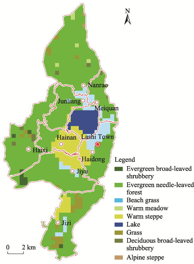
Fig. 3 Distribution of potential vegetation types of Lashihai Watershed based on the logistic regression model
There is a total of eight potential vegetation types in the Lashihai region, excluding lakes. While the evergreen needle-leaved forest is the dominant vegetation type that is most widely distributed, the other potential vegetation types are warm meadow, grass, evergreen broad-leaved shrubbery, deciduous broad-leaved shrubbery, warm steppe, alpine steppe, and beach grass. The distribution of evergreen needle-leaved forest is concentrated in the mountains around the Lashihai region, interspersed with a few patches of other vegetation types such as warm meadow, evergreen broad-leaved shrubbery, etc. On the flat land near the Lashihai region, which is generally lacustrine terrace and lacustrine platform, there are mainly warm meadow, lakes and beach grass. In terms of the area of each potential vegetation type, the potential distribution area of the evergreen needle-leaved forest accounts for 75.67% of the whole region, while the second largest vegetation type (i.e., warm meadow) accounts for only 9.32%, the third (beach grass) accounts for 5.96%, and the other vegetation types account for less than 5% each. It should be noted that the potential lake area of the Lashihai region accounts for only 3.54% of the total region.
According to the sampling analysis of paleovegetation in the Lashihai region, which was extracted from the “Study on vegetation succession and climate change in Northwest Yunnan region since late pleistocene epoch” (Song, 2007), the vegetation of Lashihai region is needle-leaved forest dominated by pine. According to that study, the evergreen needle-leaved forest mainly includes Pinus yunnanensis pure forest, as well as Pinus densata, Quercus, and mixed masson pine and oak forest. The evergreen broad-leaved shrubbery and the undergrowth grass rarely occur, which is consistent with the potential vegetation types of the study areas determined in this study. Therefore, it is further proven that the determination of potential vegetation types in the Lashihai region in this study is reliable.
In the Fig. 4, we can see that there are a total of five potential vegetation types in the strong human interference area, i.e., evergreen needle-leaved forest, warm meadow, beach grass, lake and evergreen broad- leaved shrubbery, accounting for 65.43%, 15.24%, 11.15%, 7.06% and 1.12%, respectively. The potential distribution of evergreen needle-leaved forest in the strong human interference area forms the outermost circle of the “three-circle structure” of Lashihai ecology, and is connected with the weak human interference area, thus surrounding and protecting the ecological safety of Lashihai wetland, fishing, planting, forestry and fruit growing industries, as well as the villages and towns along the lakes. The beach grass and the warm meadow form the intermediate circle of Lashihai ecology. The beach grass is mainly located in the east of the Lashihai region, adjacent to the Lashihai Lake. The warm meadow is located in the south of the Lashihai region, mainly in the east of Hainan Village, the west of Haidong Village and the north of Jiyu Village. The distribution of potential lakes is consistent with the current situation of the Lashihai region, and is located in the center of the Lashihai region forming the core circle of the three-circle ecological structure.
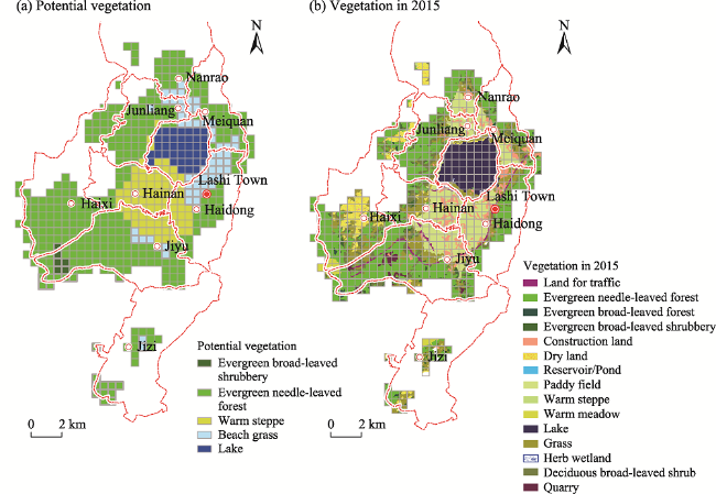
Fig. 4 Comparison of potential vegetation types in the strong human interference area vs. vegetation in 2015
A comparison of the distributions of current vegetation and potential vegetation shows that Lashihai is less disturbed by humans in the core circle; while in the intermediate circle, the area of potential beach grass has been developed into construction land, paddy field and transportation land, and the area of warm meadow has developed into paddy field and settlement; and in the outermost circle, the area of evergreen needle-leaved forest has developed into dry land and mining field, or degraded to grassland due to human influence.

4.3.2 Analysis of ecological degradation in Lashihai region

By calculating the three indexes mentioned above, i.e., degradation complexity index, degradation fragmentation index and unit area degradation index, the comprehensive ecological degradation index can be obtained (Figs. 5-6). By means of the equal spacing method, the comprehensive ecological degradation is divided into six levels, corre sponding to different degradation severities (and the corre sponding relationship is shown in Table 6. Based on these criteria, the overall ecological degradation degree of the Lashihai region is slight, and the ecological degradation is mostly below the moderate degree. The severe degradation occurs only in the individual grid cells of central Haixi Village, east of Jiyu Village, southwest of Junliang Village, and south of Meiquan Village. The moderate degradation areas are often distributed in the strong human interference area of the Lashihai region, mainly around the Lashihai Lake.
Fig. 5 Spatial distributions of degradation complexity and degradation fragmentation
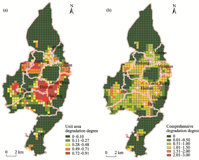
Fig. 6 Spatial distributions of unit area degradation degree and comprehensive degradation degree
Table 6 Table of ecological degradation index grading
Ecological degradation
degree
0 0.01-0.5 0.5-1.0 1.0-1.5 1.5-2.0 >2.0
Severity No degradation Slight
degradation
Mild
degradation
Moderate
degradation
Heavy
degradation
Severe
degradation
According to the statistics of ecological degradation at all degrees, the area without ecological degradation in the Lashihai region accounts for 49.86%, all of which is in weak human interference areas. In the other grades, the area with slight ecological degradation accounts for 13.05%; the area with mild ecological degradation accounts for 15.28%; the area with moderate ecological degradation accounts for 18.64%; and the area with severe ecological degradation accounts for 3.17%. Therefore, the total area at or below the mild ecological degradation degree accounts for 78.19% of the study area.

5 Discussion

In this study, the potential vegetation types are used as the reference for the original ecology of the study area to define its relatively absolute ecological degradation. The quantitative evaluation of ecological degradation is the premise and basis of ecological restoration. At present, there are many methods for the quantitative evaluation of ecological degradation, but most of them compare the ecosystem changes in a certain period through dynamic monitoring, so they lack a relatively definite degradation frame of reference. This paper makes a systematic study on the core issues and main links in degradation in the Lashihai region, such as the intensity of human disturbance, the reference frame of ecological degradation-potential vegetation and the evaluation index system of ecological degradation. The simulation of potential vegetation provides a frame of reference for the identification and evaluation of ecological degradation in Lashihai. First, the human disturbance model is used to evaluate and delineate the weak human disturbance area of Lashihai, which provides a sample area for the prediction of potential vegetation. Next, the prediction of potential vegetation types based on environmental factors is realized by Logistic regression, which better describes the primitive ecosystem of Lashihai. Finally, the degradation complexity index, degradation fragmentation index, unit area degradation index and comprehensive ecological degradation index are constructed to realize the quantitative evaluation of the ecological degradation degree based on potential vegetation. The methods used in the study have a certain reference value for the study of watershed ecological degradation and restoration on the regional scale.
Of course, there are still some shortcomings in this study. 1) The potential vegetation types are used as the reference for the original ecology of the study area to define the relatively absolute ecological degradation. However, the climate affecting the potential vegetation distribution is likely to change, and only 36 years of data from 1980 to 2015 were used for the potential vegetation simulation, so the period of time is relatively short. 2) Most of the other environmental factors are based on the data of single year around 2004, therefore, the potential vegetation results based on the simulation have a lack of stability. 3) The environmental factor dataset used for potential vegetation prediction does not contain lighting data, and the calculation model of the evapotranspiration data products does not consider the influence of topography on lighting, hence the factors used for potential vegetation prediction are not comprehensive enough, so the simulation of some light-sensitive vegetation types may not be accurate enough. 4) The ecological interference of the Lashihai region is relatively weak, and there is a difference between the strong interference area and the weak interference area. Therefore, if this method is applied to other areas with particularly strong human interference, its applicability may be reduced. For example, if the method is used to predict the potential vegetation in the Beijing-Tianjin-Hebei region, it would be difficult to determine the vegetation types in the weak human interference area or an area without degradation.
In the future, we can also carry out in-depth research which considers several additional aspects. 1) We could use more detailed and accurate environmental factor data and vegetation data to predict potential vegetation, and obtain more reasonable and precise results of the potential vegetation prediction. 2) In a longer timescale, we could simulate the potential vegetation in each climatic period according to the climate fluctuations, and define the ecological degradation degree, so as to provide a reference for the regional vegetation restoration under the global climate change. 3) The potential vegetation prediction methods, including the Logistic regression model, could be compared and studied to determine the best model for potential vegetation prediction. 4) The applicability of the ecological degradation degree method in this paper could be further verified in other regions.

6 Conclusions

Overall, this analysis led to four main conclusions. 1) The distribution of human interference is uneven in the Lashihai region. The strong human interference areas are concentrated in the Lashihai basin, and the main influencing factors are road, settlement and cultivated land. Hainan Village, Jiyu Village, Haidong Village, Junliang Village, Meiquan Village and Haixi Village along the lakes have sustained great interference by humans. 2) The original ecology of the Lashihai region is represented by a total of eight potential vegetation types, including evergreen needle-leaved forest, warm meadow, grass, beach grass, evergreen broad- leaved shrubbery, deciduous broad-leaved shrubbery, warm steppe and alpine steppe. The evergreen needle-leaved forest is the dominant vegetation type, and it is distributed in the mountains around the Lashihai region. Lake, warm meadow and beach grass distribute in the la-custrine terrace and lacus-trine platform near the Lashihai region. 3) The most impactful factors affecting the potential vegetation distribution are elevation and average phosphorus content. Different vegetation types vary in their sensitivities to the environmental factors. For example, the evergreen broad-leaved shrubbery is sensitive to accumulated temperature above 10 ℃, organic content, elevation, etc.; the evergreen needle-leaved forest is sensitive to the slope aspect, phosphorus content and organic content; and the warm meadow is sensitive to almost all environmental factors. 4) The overall ecological degradation degree of the Lashihai region is slight, the ecological degradation is mostly at or below the mild degree (78.19%), and the area without ecological degradation accounts for a high proportion (49.86%). In the three-circle structure of Lashihai ecology, there are patches of local degeneration and spotty degeneration in the outermost circle, and the potential evergreen needle-leaved forest is degenerated into grass and dry land. The intermediate circle (i.e., distribution area of warm meadow and pit-pond reservoir) is characterized as overall occupation, extensive planting, spotty development, water retreating and grass advancing, and limited survival. Finally, the water area of the core circle is slightly expanded compared with its potential state.
[1]
Bunn S E, Davies P M, Mosisch T D. 1999. Ecosystem measures of river health and their response to riparian and catchment degradation. Freshwater Biology, 41(2): 333-345.

DOI

[2]
Collado A D, Chuvieco E, Camarasa A. 2002. Satellite remote sensing analysis to monitor desertification processes in the crop-rangeland boundary of Argentina. Journal of Arid Environments, 52(1): 121-133.

DOI

[3]
Du X, Gao X M, Ma K. 2003. Diagnosis of ecosystem degradation degree: Basis and premise of ecological restoration. Chinese Journal of Plant Ecology, 27(5): 700-708. (in Chinese)

DOI

[4]
Echeverría C, Kitzberger T, Rivera R, et al. 2011. Assessing fragmentation and degradation of dryland forest ecosystems. Principles and Practice of Forest Landscape Restoration, (1): 65-102.

[5]
Gachene C K K, Mungai D N, Stahl M, et al. 1993. Land degradation in East Africa. AMBIO, 22(8): 505-508.

[6]
Hu Y F, Han Y Q, Zhang Y Z, et al. 2017. Extraction and dynamic spatial-temporal changes of grassland deterioration research hot regions in China. Journal of Resources and Ecology, 8(4): 352-358.

DOI

[7]
Jahani A, Feghhi J, Makhdoum M F, et al. 2016. Optimized forest degradation model (OFDM): An environmental decision support system for environmental impact assessment using an artificial neural network. Journal of Environmental Planning and Management, 59(2): 222-244.

DOI

[8]
Ma L G, Cao Y R, Li X T. 2011. Assessment of ecosystem health in Lashihai Lake using AHP method. Journal of Geo-Information Science, 13(2): 234-239. (in Chinese)

DOI

[9]
Li H P, Du J Q, Tang H J. 2021a. Estimation of soil organic carbon density and reserves based on random forest model in county level. Soil and Fertilizer Sciences in China, (3): 1-8. (in Chinese)

[10]
Li H P, Wang N P, Dai Y T. 2021b. Distribution of bird density in Lashihai Lake under different intensities of human activities. Wetland Science, 19(2): 162-169. (in Chinese)

[11]
Li H P, Wang N P, Dai Y T. 2021c. Spatial distribution of human activity intensity in Yunnan-Guizhou Plateau Wetland scenic area: A case study of Lashihai watershed in Yunnan Province, China. Chinese Journal of Applied Ecology, 32(8): 2915-2922. (in Chinese)

[12]
Liu G, Fu B J. 2000. Major types, characteristics and distribution of ecological degradation in China. Acta Ecologica Sinica, 20(1): 13-19. (in Chinese)

[13]
Ouyang Z Y, Zhang L, Wu B F, et al. 2015. An ecosystem classification system based on remote sensor information in China. Acta Ecologica Sinica, 35(2): 219-226. (in Chinese)

[14]
Peng S L. 2007. Restoration ecology. Beijing, China: Meteorological Press. (in Chinese)

[15]
Ren Z C, Zhu H Z, Shi H, et al. 2020. Spatio-temporal distribution pattern of potential natural vegetation and its response to climate change from Last Interglacial to future 2070s in China. Journal of Natural Resources, 35(6): 1484-1498. (in Chinese)

DOI

[16]
Sinclair A H, Moldenhauer W C, Hudson N W. 1988. Conservation farming on steep lands. Journal of Applied Ecology, 27(2): 766-767.

DOI

[17]
Song X Y. 2007. Late Pleistocene vegetation succession and climatic change in northwestern Yunnan, China. Diss., Beijing, China: Institute of Botany, Chinese Academy of Sciences. (in Chinese)

[18]
Suding K, Higgs E, Palmer M, et al. 2015. Committing to ecological restoration. Science, 348(6235): 638-640.

DOI

[19]
Tian M R, Gao J X, Zou C X, et al. 2016. Theories, ideas and methods for diagnosis of ecological degradation in important ecological function areas. Journal of Ecology and Rural Environment, 32(5): 691-696. (in Chinese)

[20]
Wu D H. 1978. Study on reasons of grassland degradation and corresponding restoration approaches. Journal of Southwest Minzu University (Natural Science), (1): 41-48. (in Chinese)

[21]
Zhu J J, Li F Q. 2007. Forest degradation/decline: Research and practice. Chinese Journal of Applied Ecology, 18(7): 1601-1609. (in Chinese)

Outlines

/