Animal Ecology

How Snow Leopards Share the Same Landscape with Tibetan Agro-pastoral Communities in the Chinese Himalayas

  • XIAO Changxi , 1, 2, 3 ,
  • BAI Defeng 1, 2 ,
  • Joseph P. LAMBERT 1 ,
  • LI Yibin 3 ,
  • Lhaba CERING 4 ,
  • GONG Ziling 2, 5 ,
  • Philip RIORDAN 1, 6 ,
  • SHI Kun , 1, 3, *
Expand
  • 1. Wildlife Institute, School of Ecology and Nature Conservation, Beijing Forestry University, Beijing 100083, China
  • 2. Everest Snow Leopard Conservation Center, Rikaze, Tibet 857000, China
  • 3. Eco-Bridge Continental, Beijing 100085, China
  • 4. Qomolangma National Nature Reserve Administration, Rikaze, Tibet 857000, China
  • 5. Vanke Foundation, Shenzhen, Guangdong 518000, China
  • 6. Marwell Wildlife, Winchester SO21 1JH, UK

XIAO Changxi, E-mail:

Received date: 2021-04-16

  Accepted date: 2574-07-12

  Online published: 2022-04-18

Abstract

The snow leopard (Panthera uncia) inhabits a human-altered alpine landscape and is often tolerated by residents in regions where the dominant religion is Tibetan Buddhism, including in Qomolangma NNR on the northern side of the Chinese Himalayas. Despite these positive attitudes, many decades of rapid economic development and population growth can cause increasing disturbance to the snow leopards, altering their habitat use patterns and ultimately impacting their conservation. We adopted a dynamic landscape ecology perspective and used multi- scale technique and occupancy model to better understand snow leopard habitat use and coexistence with humans in an 825 km2 communal landscape. We ranked eight hypothetical models containing potential natural and anthropogenic drivers of habitat use and compared them between summer and winter seasons within a year. HABITAT was the optimal model in winter, whereas ANTHROPOGENIC INFLUENCE was the top ranking in summer (AICcw≤2). Overall, model performance was better in the winter than in the summer, suggesting that perhaps some latent summer covariates were not measured. Among the individual variables, terrain ruggedness strongly affected snow leopard habitat use in the winter, but not in the summer. Univariate modeling suggested snow leopards prefer to use rugged land in winter with a broad scale (4000 m focal radius) but with a lesser scale in summer (30 m); Snow leopards preferred habitat with a slope of 22° at a scale of 1000 m throughout both seasons, which is possibly correlated with prey occurrence. Furthermore, all covariates mentioned above showed inextricable ties with human activities (presence of settlements and grazing intensity). Our findings show that multiple sources of anthropogenic activity have complex connections with snow leopard habitat use, even under low human density when anthropogenic activities are sparsely distributed across a vast landscape. This study is also valuable for habitat use research in the future, especially regarding covariate selection for finite sample sizes in inaccessible terrain.

Cite this article

XIAO Changxi , BAI Defeng , Joseph P. LAMBERT , LI Yibin , Lhaba CERING , GONG Ziling , Philip RIORDAN , SHI Kun . How Snow Leopards Share the Same Landscape with Tibetan Agro-pastoral Communities in the Chinese Himalayas[J]. Journal of Resources and Ecology, 2022 , 13(3) : 483 -500 . DOI: 10.5814/j.issn.1674-764x.2022.03.013

1 Introduction

Wildlife and local people do not always confront each other with intolerance (Heltai, 2013; Sarmento and Reading, 2016; Sullivan et al., 2018). Even with large predators such as spotted hyena (Crocuta crocuta) and common leopards (Panthera pardus), peaceful coexistence with people can occur (Yirga et al., 2013; Braczkowski et al., 2018). The snow leopard (Panthera uncia) is a cryptic apex predator of Central Asia and the Himalayan mountain landscape ecosystem (Jackson, 1996), where pastoralists and snow leopards have a long history of interaction and coexistence (Mishra et al., 2016). In the Tibetan and other Buddhist regions, snow leopards have long received culturally-based tolerance (Li et al., 2014; Suryawanshi et al., 2014; Sharma et al., 2015; Chen et al., 2016). Reported livestock depredation events by snow leopards have occurred much less frequently than those by other sympatric large carnivores such as wolf (Canis lupus) and lynx (Lynx lynx) in the Tibetan communities near the northern side of Mount Qomolangma (known as Mt. Everest) (Chen et al., 2016).
These benign relations between wildlife and humans may not attract as much public attention as direct conflicts, which often manifest as retaliatory killings in response to human deaths and economic losses (Treves and Karanth, 2003; Packer et al., 2005). However, alongside the rapid increases in economic development and population size, such a delicate relationship can easily be disturbed, threatening both snow leopards and the livelihoods of those living in remote and inaccessible mountains. Further understanding snow leopard habitat use in the context of landscape ecology, and how the species shares the same mountain landscape with humans, can highlight positive steps towards greater coexistence elsewhere.
Because landscapes contain mosaics of habitat patches (Dunning et al., 1992), an adequate landscape for a particular species may contain a mixture of habitat patches in order to provide sufficient resources. In reality, resource patches are unlikely to be uniformly distributed in space and time. The success of individual animals strongly depends on their ability to optimize resource usage spread across habitat patches (Hilty et al., 2019). However, increasing human activities and development in the Himalayas and Tibetan Plateau have gradually modified and eroded the natural landscapes' relative integrity, and consequently altered snow leopard resource usage (Miehe et al., 2014; Li et al., 2016). These changes produce more mosaic fragments and restrict the wildlife and locals to smaller communal patches of unevenly distributed and limited resources, accelerating and intensifying existing competition (Pandit et al., 2014; Dias et al., 2020). This scenario has impacted solitary wild felids directly and indirectly, which require large, unfragmented habitats of good quality to survive (Sunquist and Sunquist, 2001). However, these latent interactive mechanisms between human-predator-landscape may be easily overlooked in the case of minor or inconspicuous conflicts. For example, we still know little about how snow leopards use these environments or how that usage varies seasonally under human influences.
A robust and simple methodology for assessing snow leopard habitat use in such a challenging environment and with limited resources is indispensable. Occupancy models and the techniques of landscape ecology are two such methodologies (Mackenzie et al., 2002; Alexander et al., 2016a; Robinson and Weckworth, 2016). Occupancy modeling is a powerful tool for examining rare and elusive species, especially due to the model's adjustable detection probabilities for habitat use status and trends for infrequently encountered species with large home ranges (Mackenzie et al., 2002; Alexander et al., 2016a). Landscape ecology offers a dynamic organism-centered scope rather than a static or anthropocentric view (McGarigal et al., 2016). It places a great deal of importance on defining appropriate scales on a shared landscape in order to analyze habitat patch use, often expressed as grain, which describes the geographical or temporal resolution of an ecological process occurring within habitat patches (Nyhus et al., 2016).
Furthermore, all biological processes relating to a particular organism occur at different spatial scales and across varying time scales. The spatial and temporal scales at which landscape variables are examined should fit the organism's characteristics, such as their movement and environment, to answer questions pertaining to the species' habitat use and its relation with variables related to spatial and temporal variations.
Compared with other carnivores, relatively few studies of snow leopards have explicitly applied a landscape ecology perspective (Alexander et al., 2016a; Riordan et al., 2016; Robinson and Weckworth, 2016; Atzeni et al., 2020). Previous studies mainly used a single scale of terrain-related variables predetermined by the Digital Elevation Model (DEM) resolution, an approach which places invariable a priori constraints on the responses of highly mobile large carnivores to the environment. However, the pattern of patches varies with spatial extent and scale, as do the resource mosaics used by snow leopards (Robinson and Weckworth, 2016). Without attempting to establish the best scales for each covariate empirically, the pre-selected variables probably lead to bias in the occupancy model because they do not fully consider the species characteristics that are related to the specific habitat background. Environmental and anthropogenic variables that affect snow leopard habitat use have been reported in many occupancy studies. However, seasonal variations and the complex quantitative interactions between covariates have not been fully reported. This lack of research may hamper conservation efforts, such as nature reserve management after long periods of rapid social-economic development, especially for large carnivores and rural communities in the vulnerable alpine environment of the Himalaya or Qinghai-Tibetan Plateau.
Qomolangma National Nature Reserve (QNNR) adjoins the Himalayas and Qinghai-Tibetan Plateau, and has been identified as a valuable area with large suitable habitat that might provide a climate refuge for snow leopard populations in the next 50 years (Forrest et al., 2012; Li et al., 2016; Riordan et al., 2016; Bai et al., 2018). It is an important natural route for the connectivity of snow leopard habitat patches along the high Himalaya, which is vital for maintaining healthy gene flow of the regional snow leopard populations because it is near the national border (Riordan et al., 2016). The area has been assessed as being in or adjoining several snow leopard conservation units with the highest priority after a series of international symposia and conservation studies, such as SLCUs (McCarthy et al., 2016), SLLs (Snow Leopard Working Secretariat, 2013), and LCUs (Li et al., 2020). Despite this importance, there is a notable lack of studies both at the global scale and in regional snow leopard ranges like Himalaya or Qinghai-Tibetan Plateau (Alexander et al., 2016b; Riordan et al., 2016; Snow Leopard China, 2019).
In this study, we carefully explored the habitat use of snow leopards and systematically surveyed how they share this landscape with rural Tibetan communities in the QNNR of China's Tibetan Autonomous Region (TAR) in the central Himalaya's northern slope. We used a single-season, multi-scale occupancy model (Mackenzie et al., 2002) to determine the environmental and anthropogenic variables with variations between seasons for the presence and the detection of snow leopards. We created eight habitat use models based on landscape ecology, analyzed the effective extent of different covariates with multi-scales for habitat use of snow leopards, and examined how these covariates affected each other and the realistic difficulties in the selection and measurement of the variables.

2 Method

2.1 Study area

The research was conducted in one of the world's highest reserves, Qomolangma National Nature Reserve (QNNR). QNNR (33819 km2, 27°48° to 29°12° N; 84°27° to 88°21° E) occupies a unique geographic position, lying on the north side of the central Himalayas at the border of China's Tibetan Autonomous Region and Nepal. Its southern edge borders five Nepalese protected areas. QNNR includes four administrative counties in total, and the research was conducted in Dingri County. The dominant ecosystem in Dingri is high altitude alpine and cold desert, with an average altitude of about 4500 m (Wang et al., 2013), making it even higher than the Spiti valley (Singh et al., 2019) in trans-Himalaya, which is one of the famous highlands for snow leopard research in India. Our study area comprises two townships of Dingri County, both with very high baseline elevations (>4200 m), containing about 74% of the administrative villages (38 total, 2010) and including approximately three-quarters of the county's population (10331 total, 2017). Livestock husbandry is one of the primary sources of livelihood and a vital component of the economy of these villages. A few fluvial plains in the lower elevations make construction and cultivation easier than in the highly rugged uplands. Most of the villages and roads were located along rivers or streams in the bottom of large gullies. Paved or unpaved roads in our survey grids linked all the villages.

2.2 Survey design

The surveyed landscape was divided into 33 standard array grid cells of 5 km×5 km each (Hines et al., 2010; Bailey et al., 2014), with eight rows and seven columns totaling 825 km2, based on the published home range of snow leopards (Jackson et al., 2014). A total of 118 cameras (113 Ltl Acorn and 5 RECONYXTM) were systematically deployed in 31 grid cells. These cells were chosen to exclude the main traffic road, dense townships, and expansive flat semi-arid river beds, which were thought to be unfavorable habitats for snow leopards (Riordan et al., 2016) (Fig. 1).
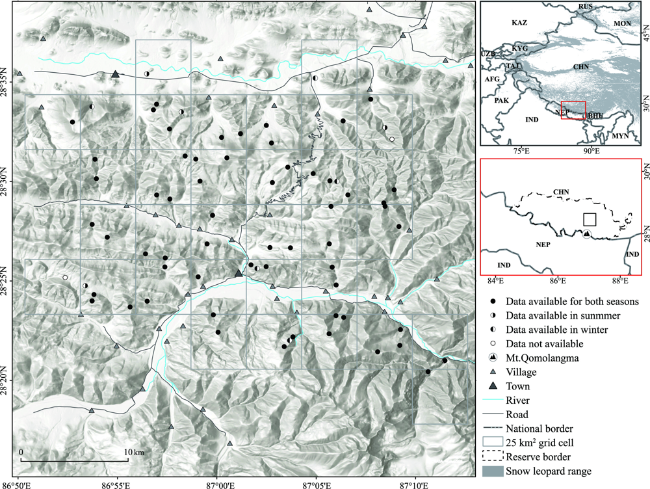
Fig. 1 Location of study area and map of the camera-trap surveyed areas (sites) used to model snow leopard (Panthera uncia) habitat use for summer and winter in Qomolangma NNR, China.

Notes: Country names are abbreviated: Afghanistan (AFG); Bhutan (BHU); China (CHN); India (IND); Kazakhstan (KAZ); Kyrgyzstan (KYG); Mongolia (MON); Myanmar (MYN); Nepal (NEP); Pakistan (PAK); Russia (RUS); Tajikistan (TAJ); Uzbekistan (UZB). Projection: UTM45 N; Datum: WGS 1984.

Two teams conducted the surveys, each with at least one person trained in using camera traps (e.g., a staff member from the reserve or field researcher) and one local guide. We left a minimum Euclidean distance of 1-1.5 km between each station to assure independence and reduce spatial auto-correlation, except for three sections which had camera distances of less than 600 m due to their accessibility. The specific camera-trap stations were chosen to maximize the possibility of detecting snow leopards in each transect. Transects of at least 5 km in length were selected in each grid cell based on accessibility. Areas with a high probability of snow leopard presence along each transect were chosen for camera trap stations based on the known snow leopard habitat preferences. We chose stations with features such as mountain ranges, the base of cliffs, animal trails, highly rugged terrain, and abundant prey resources (Fox et al., 1991; Jackson, 1996; Jackson and Hunter, 2003; McCarthy and Chapron, 2003). Snow leopard signs, including feces, scrapes, pugmarks, urine, and scent markings, were identified and recorded to determine the best locations for the camera traps. At each station, two cameras were set, face-to-face at a slight angle. This was done to obtain photographs of the snow leopards from both sides and avoid interference from the other camera's light. Our camera trap set up elevation was quite high due to the high average altitude of study area (mean=4710 ± SD 314 m, range 3958- 5324 m). Cameras were operational between October 2017 and November 2018. Memory sticks and batteries were checked in the middle of June 2018. All cameras were programmed to operate for 24 h d-1.

2.3 Data analysis

2.3.1 Overview of the modeling framework

In general, five main steps were adopted for the entire modeling process in this study. 1) We built two detection histories of the snow leopard in the coldest and warmest periods of a year. 2) We adopted a multiple-scale approach to model the gradient variables that account for a differential landscape perception of snow leopards as a function of seasonality. We also examined different methods for measuring the conventional anthropogenic covariates to test the fitness in a complex landform in different seasons. 3) Then, according to the covariate candidates selected in the previous step, we developed eight hypothetical habitat use models for the two seasons based on field observations and the literature. 4) Subsequently, we ranked the univariate models to select the optimum covariates from among the candidates in step two, decreasing the risk of model overestimation. Meanwhile, we employed the true multiple-scale technique and compared its outcomes with the univariate model results for mutual authentication in order to find the most appropriate gradient covariates. 5) On the basis of the final variable candidates from step four, we used the single-season occupancy model to explore the above eight presumptive models for establishing and calculating the estimates of the probability of snow leopard presence and detection. The sub-steps of each process are elaborated in the following sections.

2.3.2 Detection history

The total detection history was split into two separate seasons of 90 days each. This length was chosen to reduce the violation of the model closure assumption risk. The two seasons, winter and summer, were chosen to align with the typical alpine climate in which the seasons of spring and autumn are short and unapparent. We hypothesized that the snow leopard activity pattern is distinct between the harsh winter with the lowest temperature and precipitation (Nov. 2017-Jan. 2018), and the warm summer with much more rainfall (May-Jul. 2018).
Detection histories were expressed as multi-day periods to increase the overall detectability of snow leopards. For each survey site, each 90-day season was separated into four different scenarios (5-day, 10-day, 15-day, and 18-day periods) corresponding to four different sampling occasions (18, 9, 6, and 5, respectively). The goodness-of-fit (GoF) of each scenario in each season was assessed with the most complex model (global model), and only the optimum scenario was retained (MacKenzie and Bailey, 2004).

2.3.3 Candidate covariate set

The topographic features represent a landscape character of heterogeneity in the study area and are relevant to the snow leopard's ecology, and the appropriate “scales” were selected for describing most ecological applications (Cushman et al., 2010) of snow leopards (e.g., patch use) within an individual's home range (Robinson and Weckworth, 2016). Gradient landscape variables were considered, including elevation (ELE), slope (SLP), and terrain ruggedness (TRI) (Li et al., 2014; Alexander et al., 2016a). Considering the appropriate scale is not as simple as looking at the dimensions of the study area (Robinson and Weckworth, 2016). These variables were measured at a variety of spatial scales (Wu, 2007), with the focal radius ranging from 30 to 4000 m in a gradient (30 m, 300 m, 1000 m, 2000 m, and 4000 m separately) for sufficient spatial heterogeneity (Johnson, 1980). Multiple scale values of elevation (ELE), slope (SLP), and terrain ruggedness index (TRI) were generated from a Digital Elevation Model (DEM, www.gscloud.cn) with 30 m×30 m resolution using the tools of Roughness and Mean Slope, in Geomorphometry and Gradients Metrics of ArcGIS (10.2, ESRI).
The impacts of potentially fragmenting landscape features (i.e., linear or graphic landscape elements, such as roads or villages) were considered, because the rapidly growing population and tourism industry in the study area (Chen et al., 2017) has increasingly fragmented the potential snow leopard habitat. However, the impacts of fragmenting features might be reduced at increasingly coarse spatial scales due to the relatively simple traffic networks, the small-scale rural residential communities and the strong diffusion capacity of snow leopards (Jackson, 1996). Two different methods were adopted for measuring disturbance from human settlements (SETT) and roads (ROAD). In the first one, we used the shortest Euclidean distance (Dist.) between each site and either a point representing a settlement (Dist._SETT) or a line representing a road (Dist._ ROAD) (Alexander et al., 2016a). In the second method, we used kernel density (KD) functions to measure the strength and range of influence of human settlements (KD_SETT) or roads (KD_ROAD) (Atzeni et al., 2020). Specifically, the road network (Fig. 1) in the study area is formed by five main roads with smaller sub-road structures with different levels of use. Each road was weighted by categorizing it into one of three grades indicating traffic flow (from 1-3, where 1 indicates lowest traffic flow and 3 indicates highest) according to open source (Open Street Map). Human settlements (Fig. 1) were also given two weighting values to categorize them as either village (weighted with 1) or township (weighted with 2).
Prey resources was considered a key variable impacting snow leopard habitat use (Alexander et al., 2016a). Blue sheep (Pseudois nayaur) is the main prey resource for snow leopard in the Tibetan plateau and central Himalayas (Schaller 1998; Nyhus et al., 2016). Blue sheep capture rates (BS) were calculated from camera trap photos by dividing the number of independent events (≥30 min) containing blue sheep by the total number of active camera trap days (i.e., number of days for which the specific camera station was active). Other potential prey vertebrates were also detected, such as Himalayan musk deer (Moschus leucogaster), Himalayan marmot (Marmota himalayana), and woolly hare (Lepus oiostolus). However, they were not detected frequently enough to be incorporated into our model.
Livestock grazing is the main source of livelihood for the local inhabitants and represents the anthropogenic influence outside of the concentrated human settlements. We estimated grazing activity rate (GRAZE), which was calculated in the same way as blue sheep capture rates (BS), but based on detections of livestock. The local livestock included sheep (Ovis aries), goat (Capra aegragus), donkey (Equus africanus asinus), horse (Equus ferus caballus), yak (Bos grunniens), and cattle (Bos taurus), although no cattle were detected during the survey periods.
In total, 21 types (with multiple scales or distinct measurement methods) of habitat use (ψ) candidate covariate sets were included in each season (Table 1).
Table 1 Candidates of snow leopard (Panthera uncia) habitat use (ψ) covariates
Category Covariate Detail Abbreviation
Environmental covariates Blue sheep capture rates Camera-trap capture BS
Sites of slope gradient 30 m, 300 m, 1000 m, 2000 m, 4000 m SLP30-4000
Sites of terrain ruggedness index 30 m, 300 m, 1000 m, 2000 m, 4000 m TRI30-4000
Sites of elevation 30 m, 300 m, 1000 m, 2000 m, 4000 m ELE30-4000
Anthropogenic covariates Grazing activity rates Camera-trap capture GRAZE
Disturbance from human settlements Kernal density KD_SETT
Distance of the nearest Dist._SETT
Disturbance from traffic roads Kernal density KD_ROAD
Distance of the nearest Dist._ROAD
We included a binary covariate to indicate which of the two survey teams placed a particular camera trap (TEAM) and incorporated it into our detection probability models (p) to account for potential observer bias and differences between the two teams.

2.3.4 Development of the hypothetical habitat use model

Eight hypothetical habitat use models were developed with potential covariates of site use probability (ψ) and detection probability (p) for each season (Table 2). 1) The NULL model, with the constant detection and site use probability, assumed habitat use of snow leopard was unaffected by any of the observed variables. 2) The model PREY contained the variable of blue sheep camera-trap capture rates (BS). It represented the hypothesis that snow leopard habitat use is strongly dependent on the presence of blue sheep as their primary food resource. 3) Five scale-variant versions of the model TOPOGRAPHY included measures of terrain ruggedness index (TRI), slope (SLP), and elevation (ELE) at multiple scales, based on the hypothesis that snow leopards prefer to use high, rugged terrain with steep cliff edges. 4) The model HABITAT included all potential topographic variables from the third model and the blue sheep capture rates (BS). This model assumed that snow leopards use the rugged mountain crest habitat where prey is abundant. 5) A model of ANTHROPOGENIC INFLUENCE was developed to represent the assumption that snow leopards avoid areas with high levels of human disturbance. This model included the variables of grazing activity rates (GRAZE), human settlements (SETT), and roads (ROAD). The final three models were developed by combining the above anthropogenic impact factors with environmental factors. 6) A model of PREY + ANTHROPOGENIC INFLUENCE, assumed that snow leopards use habitat based on ease of access to prey while avoiding human disturbance. 7) A model of TOPOGRAPHY + ANTHROPOGENIC INFLUENCE assumed that snow leopards live in a harsh mountainous environment with less human activity. 8) The final GLOBAL model, incorporating all potential variables, assumed snow leopards use high, rugged, and steep terrain where prey is abundant with limited human disturbance.
Table 2 Description of priori candidate models describing the effects of potential environmental variables on the probability of habitat use by snow leopard (Panthera uncia)
Model name
(Abbreviation)
Covariates (Abbreviation) Hypothesis Expected
influence on ψ
Supporting literature
1 NULL N/A Snow leopard habitat use is not affected by environmental variables N/A N/A
2 PREY Blue sheep capture rates (BS) Snow leopards use habitat based on access to prey Positive Barber-Meyer et al., 2013; McCarthy, 2000; Sharma et al., 2015
3 TOPOGRAPHY (TOP.) Slope (SLP) Snow leopards use high mountain areas with rugged and steep slope terrain Positive Sunarto et al., 2012; Taubmann et al., 2016; Klaassen and Broekhuis, 2018; Ghoshal et al., 2019; Watts et al., 2019
Terrain ruggedness index (TRI) Positive
Elevation (ELE) Positive
4 HABITAT Blue sheep capture rates (BS) Snow leopards use high, steep slope, and rugged habitat where prey is abundant Positive Sunarto et al., 2012; Barber-Meyer et al., 2013; Taubmann et al., 2016; Klaassen and Broekhuis, 2018; Ghoshal et al., 2019
All potential TOP. variables Positive
5 ANTHROPOGENIC INFLUENCE (A.I.) Grazing activity index (GRAZE) Snow leopards avoid areas with high levels of human disturbance Negative McCarthy and Chapron, 2003; Cosentino et al., 2014; Lewis et al., 2015; Alexander et al., 2016a
Disturbance from human settlements (SETT) Negative
Disturbance from traffic roads (ROAD) Negative
6 PREY+A.I. Blue sheep capture rates (BS) Snow leopards use habitat based on access to prey and avoiding human disturbance Positive McCarthy, 2000; McCarthy and Chapron, 2003; Alexander et al., 2016a
All potential A.I. variables Negative
7 TOP.+A.I. All potential TOP. variables Snow leopards use rugged, high elevation habitat with little human disturbance Positive Sunarto et al., 2012; Alexander et al., 2016a; Klaassen and Broekhuis, 2018; Ghoshal et al., 2019
All potential A.I. variables Negative
8 GLOBAL Blue sheep capture rates (BS) Snow leopards use high elevation, rugged habitat where prey is abundant and with low human disturbance Positive McCarthy and Chapron, 2003; Sunarto et al., 2012; Taubmann et al., 2016; Ghoshal et al., 2019
All potential TOP. variables Positive
All potential A.I. variables Negative

Note: All models are based on hypotheses developed from the cited supporting literature. The models shown here are before removing correlated variables, and those which were non-optimum candidates at the stage of the univariate habitat modeling and true multi-scale evaluation. For the full model set included in the final analysis, see Table 3. No paremeters (N/A).

Table 3 Description of a priori candidate models describing the effects of environmental variables on the probability of habitat use by snow leopard (Panthera uncia)
Covariate (unit) Abbreviation (scale) Relationship to snow
leopard occurrence
Season Effective sample
range (mean±SD)
Station ratio
recorded to target
Supporting literature
Grazing activity
capture rate index (%)
GRAZE (N/A) Avoids sites with high levels of human disturbance Winter 0-54.55 (7.59±10.24) 88.53 McCarthy and Chapron, 2003; Alexander et al., 2016a
Summer 0-67.78 (14.71±16.44) 95.16
Blue sheep capture rate index (%) BS (N/A) Habitat use based on access to prey Winter 0-36.67 (2.80±5.6) 47.54 McCarthy, 2000; Barber-Meyer et al., 2013; Sharma et al., 2015
Summer 0-20.45 (2.14±3.66) 50.77
Slope of sites (°) SLP (1000) Uses certain steep habitat Winter 15.93-32.70 (22.15±3.17) N/A Sunarto et al., 2012; Klaassen and Broekhuis, 2018
SLP (1000) Summer 7.49-32.70 (22.03±3.77)
Terrain ruggedness index (N/A) TRI (4000) Uses rugged terrain habitat Winter 12.11-21.36 (15.50±1.96) N/A Taubmann et al., 2016; Ghoshal et al., 2019
TRI (30) Summer 1.40-4.09 (2.34±0.57)

Note: All models are based on hypotheses developed from the cited supporting literature. No paremeters (N/A).

2.3.5 Univariate habitat modeling and multi-scale selection

We calculated the Pearson's correlation coefficient for each pair of continuous variables at all different scales. Any pair of covariates exhibiting correlation coefficients |r|>0.6 were treated as highly collinear, however cognate variables with different scales or measurements were regarded as one category. Better univariate habitat use model performance (AICc ranking) was retained among all correlates (Tan et al., 2017). The true multiple-scale optimization approach (McGarigal et al., 2016) was conducted for comparing the outcome of topographic gradient variables with the results of the univariate model. All continuous variables were standardized to z-scores (z=(x$\bar{x}$)/|SD|) prior to modeling.

2.3.6 Occupancy modeling

A simple single-season, single-species occupancy model (Mackenzie et al., 2002) was applied using PRESENCE v. 2.12.37 (Hines, 2006) to estimate snow leopards' occupancy and detection probability. Akaike's Information Criterion corrected for small sample sizes (AICc; MacKenzie et al., 2006) was used to rank the models. Due to the large home range of snow leopards, the occupancy parameter (ψ) is interpreted in this study as site use or habitat use for a small study area, rather than site occupancy per se.
A two sub-step habitat use modeling procedure was employed. Firstly, detection probability (p) models were assessed while all habitat use covariates remained constant. The results were ranked with the corrected relative difference in Akaike's Information Criterion (∆AICc) and model weights. Afterward, the most significant contributing detection model was retained and applied in the subsequent selection of habitat use models with site covariate candidates (Long et al., 2011; Tan et al., 2017).

2.4 Model assessment

To ensure that the models in our set could be reliably interpreted, we performed a chi-squared probability (χ2p) goodness-of-fit (GoF) test on the global model (ɑ = 0.05, bootstrap permutations = 10000). This test produces an estimate of c-hat (ĉ), a measure of overdispersion, which should be close to 1 in well-fitting models (MacKenzie and Bailey, 2004). The eight hypothetical models in each season were ranked based on AICc, and models with ∆AICc≤2 were regarded as considerably supported candidates and retained for further interpretation (Strampelli et al., 2018).

3 Results

After collapsing the two 90-day detection periods into dif-ferent scenarios, the 15-day period showed the optimum performance in winter (ĉwinter = 1.08, χ2pwinter = 0.23), while the 18-day period represented the optimum in summer (ĉsummer = 1.01, χ2psummer = 0.25) (Table S1). Meanwhile, our global model fit the field data sufficiently well for us to trust all further nested models in this analysis (Table S1). In winter, snow leopards were detected 29 times at 17 of the 61 sites and on 350 occasions from 7933 camera trap days. In summer, snow leopards were observed 23 times at 15 of the 62 sites and on 310 occasions from a total of 7579 camera trap days. Except for the valid number of cameras, all other parameters had higher values for the winter data (e.g., functioning camera sites, camera working days, survey occasions, capture events, and site use naïve estimates) than for the summer data.
Average probabilities of habitat use (ψ) and detection (p) in winter were 0.44±0.11 and 0.19±0.05, respectively, and 0.45±0.18 and 0.19±0.06, respectively, in summer (Table S2). The naïve estimate of habitat use (ψ) in winter and summer underestimated occupancy by 57% and 87.5%, respectively (Fig. 2).
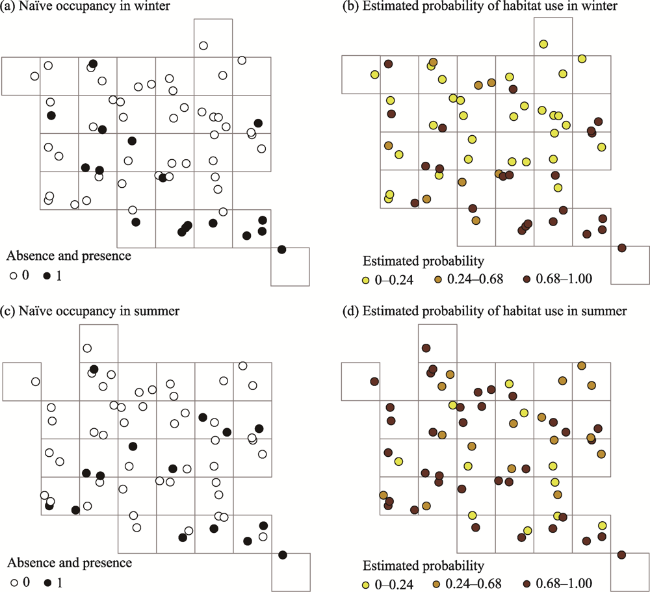
Fig. 2 Probability of site use by snow leopards (Panthera uncia), as measured by camera-traps in Qomolangma NNR, China. (a, c) Naïve estimates from a presence vs. absence approach of two seasons; (b, d) Mean estimated probabilities of habitat use of two seasons.

Note: Each cell is 5 km×5 km=25 km2.

3.1 Covariate selection

3.1.1 Correlation analysis

There were 12 and 16 pairs of correlated variables in winter and summer, respectively (Tables S3, S4). Furthermore, correlations were considered between all cognate variables (i.e., scale variant variables, such as all TRI or ELE, etc.), regardless of the values of collinearity coefficients. The remaining covariates were not strongly co-linear. All Pearson correlation coefficients were |r|<0.55 in winter and |r|<0.41 in summer.

3.1.2 Detection covariates

According to the null models, detection probabilities (p) in winter and summer were 0.24 and 0.25, respectively. The detection model including the variable of TEAM performed better than the null in both winter and summer (Table 4). The probability of detection (p) was strongly effected (AICcw) by the survey variable (TEAM) in both winter and summer (βwinter = 1.41 ± 0.59; βsummer= 1.37 ± 0.67).
Table 4 Snow leopard (Panthera uncia) detection probability models (p) in winter and summer
Models_winter AICc ∆AICc AICcw Model likelihood K -2 log LL
p(TEAM) 185.15 0 0.7917 1 3 178.73
p(.) 187.82 2.67 0.2083 0.2632 2 183.61
Models_summer AICc ∆AICc AICcw Model likelihood K -2 log LL
p(TEAM) 150.5 0 0.6857 1 3 144.09
p(.) 152.06 1.56 0.3143 0.4584 2 147.86

Note: Akaike's information criterion corrected for finite sample sizes (AICc). The relative difference in AICc values compared with the top-ranked model (ΔAICc), model weight (AICcw), Model likelihood, number of parameters (K), and -2log-likelihood (-2 log LL). The detection covariate was observer bias of camera station setting teams (TEAM). The dataset was limited to 90 sampling days with a 15-day collapsing scenario, 61 valid camera-trap stations in winter, and an 18-day collapsing scenario, 62 valid camera-trap stations in summer.

3.1.3 Covariates in univariate modeling and true multi-scale modeling

We retained the better covariates among the correlates, based on their performance in univariate habitat use models, i.e., those with lower AICc (Table S5). Generally, regarding AICc and AICcw, the terrain-related variables had better performance than the other covariates in univariate models (e.g., SLP and TRI). However, the performance of elevation (ELE) at all scales was poor. The covariates related to traffic (ROAD) and human settlement (SETT) did not perform well. The two measurements of Euclidean distance (Dist) and kernel density (KD) for human settlements and roads were both unstable. Their inclusion would increase the risk of model overestimations, and therefore, these variables were dropped from the candidate set. The final covariates retained in the univariate model section were: slope (SLP), terrain ruggedness (TRI), grazing activity (GRAZE), and blue sheep capture index rates (BS) (Table 3).
For multi-scale selection of terrain-related gradient variables, we used the results of the true multi-scale models (Table S6) to confirm the outcomes of univariate modeling (Table S5), and vice-versa. The best combinations of the two methods were both SLP1000 + TRI4000 in winter and SLP1000 + TRI30 in summer, separately. This suggests that our multi-scale selection process and results were reliable.

3.1.4 Final variable set for the hypothetical habitat use models

The final site use covariates for inclusion in the eight hypothetical models were grazing activity (GRAZE), blue sheep capture rate (BS), slope steepness with 1000 m radius in both winter and summer (SLP1000), and terrain ruggedness with radius 30 m in winter and 4000 m in summer (TRI4000 and TRI30) (Table 3). The covariate details are elaborated in the following section.

3.2 Hypothetical snow leopard site use models

Generally, the results of our proposed models suggest the probability of snow leopard habitat use differed in many respects along with seasonal variations (Table 5). Winter models showed a clearer pattern. Most of them perform much better than null and all include topographic variables, which suggested terrain-related variables were important. In comparison, the summer models were not as easily interpreted. The value of AICc in each model was close, except for the two models with slightly higher support (AICcw), suggesting that perhaps some latent covariates might not have been fully discovered in our summer models.
Table 5 Model selection results for describing the probability of snow leopard (Panthera uncia) site use (ψ) in the cold and warm seasons
No. Models_winter AICc ∆AICc AICcw Model likelihood K -2 log LL
1 HABITAT 162.26 0 0.4155 1 6 148.7
2 TOP. 162.61 0.35 0.3488 0.8395 5 151.52
3 GLOBAL 164.55 2.29 0.1322 0.3182 7 148.44
4 TOP. +A.I. 165.04 2.78 0.1035 0.2491 6 151.48
5 A.I. 187.16 24.9 0 0 4 178.45
6 PREY 187.26 25 0 0 4 178.55
7 NULL 187.82 25.56 0 0 2 183.61
8 PREY+A.I. 189.32 27.06 0 0 5 178.23
No. Models_summer AICc ∆AICc AICcw Model likelihood K -2 log LL
1 A.I. 150.57 0 0.2152 1 4 141.87
2 TOP. 150.68 0.11 0.2037 0.9465 5 139.61
3 PREY+A.I. 151.59 1.02 0.1292 0.6005 5 140.52
4 PREY 151.67 1.10 0.1242 0.5769 4 142.97
5 TOP. +A.I. 151.84 1.27 0.1141 0.5299 6 138.31
6 NULL 152.06 1.49 0.1022 0.4747 2 147.86
7 HABITAT 152.70 2.13 0.0742 0.3447 6 139.17
8 GLOBAL 154.08 3.51 0.0372 0.1729 7 138.01

Note: Akaike's information criterion corrected for finite sample sizes (AICc). The relative difference in AICc values compared with the top-ranked model (ΔAICc), model weight (AICcw), Model likelihood, number of parameters (K), and -2log-likelihood (-2 log LL).

Specifically, the two top-ranking (∆AICc≤2) models in winter were HABITAT and TOPOGRAPHY (shortened to TOP.) (Table 5). These two models held the highest support (ΣAICcw=0.76), indicating that the selected covariates were reasonably important. However, these two models did not perform as well in summer, as the relative model weight of TOP. (AICcw) decreased over 40% from winter to summer.
The ranking of HABITAT seems to have been reversed between the two seasons. These two models both include two geomorphic related variables: terrain ruggedness index (TRI) and slope steepness (SLP), and their beta coefficients (βTRI, βSLP) show a positive trend throughout winter and summer, indicating the preference of snow leopard for rough terrain at a high elevation in both seasons. Furthermore, based on the ranking of univariate modeling and the true multi-scale approach (Tables S5, S6), snow leopard habitat use probability indicated variations with more specific details. In winter, models containing slope steepness (SLP) and terrain ruggedness index (TRI) were measured at broad scales of 1000 m (SLP1000) and 4000 m (TRI4000) separately, and these all performed well. In summer, optimized scales of the slope were the same as winter 1000 m (SLP1000), while the optimized terrain roughness radius was only 30 m (TRI30) at a small scale (Tables S5, S6). The mean slope steepness (SLP) was 22° and quite steady both in winter and summer. The values of mean terrain ruggedness (TRI) were 15.5 and 2.3 in winter and summer, respectively, varying with the optimum scale of each season (Table 3).
The model HABITAT was hypothesized on the snow leopards use of an ideal natural environment with all its favored terrain features like the model of TOP., as mentioned above. Furthermore, they can easily access their main prey, blue sheep (BS). Notably, however, the beta coefficients of BS (βBS) seem to reverse direction in the two seasons (Table 6). The estimated value βBS was negative in winter but positive in summer, indicating a varying relationship between covariate BS and ψ, though with a large standard error. Figure 3 shows the trends of blue sheep and snow leopard capture occasions vary with elevation in winter and summer, respectively. There were more fluctuations of elevational range in summer for both blue sheep and snow leopard, contrasting with their relatively steady trend in winter. The winter occurrence tendency of blue sheep was lower than in summer. Its elevational range in summer is wider than in winter, indicating that blue sheep prefer to stay at lower elevations in the cold season and inhabit a wider altitude range during the warmer season. The occurrence range of snow leopards is more expanded than the range of blue sheep in general.
Table 6 Estimates of the Beta coefficient (β) and standard error (SE) of each covariate of the hypothetical models
No. Models_winter βintercepte ±SE βGRAZE±SE βBS±SE βSLP1000±SE βTRI30±SE βTRI4000±SE
1 HABITAT 0.38±0.99 N/A -1.79±1.74 7.41±4.73 N/A 2.44±1.41
2 TOP. -0.27±0.75 N/A N/A 3.89±2.06 N/A 1.62±1.01
3 GLOBAL 0.32±0.95 -0.55±1.21 -1.69±1.62 6.68±4.24 N/A 2.44±1.36
4 TOP. +A.I. -0.26±0.76 -0.15±0.74 N/A 3.90±2.04 N/A 1.66±1.04
5 A.I. -0.19±0.45 -0.21±0.40 N/A N/A N/A N/A
6 PREY -0.18±0.45 N/A -0.15±0.36 N/A N/A N/A
7 NULL -0.60±0.36 N/A N/A N/A N/A N/A
8 PREY+A.I. -0.18±0.45 -0.23±0.41 -0.17±0.36 N/A N/A N/A
No. Models_summer βintercepte ±SE βGRAZE±SE βBS±SE βSLP1000±SE βTRI30±SE βTRI4000±SE
1 A.I. -0.34±0.55 -0.77±0.57 N/A N/A N/A N/A
2 TOP. -0.20±0.58 N/A N/A 0.65±0.57 0.51±0.52 N/A
3 PREY+A.I. 0.17±1.25 -0.97±0.89 1.58±2.36 N/A N/A N/A
4 PREY 0.06±0.72 N/A 0.94±1.03 N/A N/A N/A
5 TOP. +A.I. -0.38±0.56 -0.63±0.54 N/A 0.52±0.48 0.49±0.52 N/A
6 NULL -0.57±0.44 N/A N/A N/A N/A N/A
7 HABITAT -0.12±0.65 N/A -0.37±0.57 0.80±0.66 0.70±0.66 N/A
8 GLOBAL -0.35±0.59 -0.64±0.56 -0.29±0.51 0.59±0.50 0.63±0.59 N/A

Note: Grazing activity index (GRAZE), blue sheep capture rate (BS), slope steepness of sites with scale 1000 m threshold value (SLP1000), terrain ruggedness index with scale 30 m and 4000 m threshold values (TRI30, TRI4000). No paremeters (N/A).

The ANTHROPOGENIC INFLUENCE (A.I.) was the most prominent model in summer, based on AICc and AICcw ranking. It showed a negative influence on snow leopard habitat use; however, it is worth noting that the model weight (AICcw) of A.I. was zero in winter. Since it had the lowest weight (AICcw) compared with other models in winter, it can be considered as negligible in winter. This finding indicated that grazing activities strongly impacted snow leopard site use (ψ) in summer but not in winter. Nevertheless, up to 89% of camera stations detected grazing activities within the survey area in winter (versus 95% in summer) (Table 3). Only one covariate, GRAZE, was left to incorporate into the A.I. model for both seasons. Other variables such as human settlements and roads were discarded since their performance was not good enough in the univariate model section (see 3.1.3). The beta coefficients of grazing activity (βGRAZE) indicated that grazing activity negatively influences the probability of habitat use (ψ).

4 Discussion

4.1 Complex interactions of habitat use with prey and topography, and their inextricable ties with the human community

Our study found that the frequency of blue sheep captures (BS) affected snow leopard habitat use negatively in winter but positively in summer. We found that slope steepness (SLP) at a stable scale (1000 m) had a strong positive influence in winter but a weak one in summer. Seasonal movements have been observed in many herbivore species, including both wild and domestic species crossing continents due to changes in temperature, precipitation, drinkable water availability, and forage availability (Chamaillé-Jammes et al., 2009; Mobæk et al., 2009). Studies of other felids in the genus Panthera have observed their responses to variations in prey population availability (Sunquist, 1981; Bailey, 1993), a variable which could generate similar responses in snow leopards (Roberts, 1977; Schaller, 1977; Fox et al., 1991). A series of GPS collar tracking studies in the Tost Mountains of Mongolia confirmed snow leopard habitat use was consistent between seasons, presumably because its prey's distribution varied little (Johansson et al., 2015, 2018). A blue sheep habitat use study in the Nepali Himalayas indicated this wild ungulate has seasonal habitat preferences for certain landscape features conducive to foraging and escaping. This study observed that the effect of slopes varied little between seasons, and the areas of medium steepness (<40°) were most frequently used (Oli, 1996). Similar results were also reported in another study in Nepal by Filla et al. (2020), supporting our results which suggest that snow leopards have a steady preference for topographic slope in winter or summer due to the prey distribution. Furthermore, compared to the study by Oli (1996), although they used direct visual observations and we could not deploy cameras on extremely steep sites due to safety concerns, our observations still support Oli's results.
Oli (1996) also observed that blue sheep on the southern slopes of the Himalayas preferred habitats at elevations between 4200-4600 m. They avoided sites above 4800 m because of the lack of vegetation, and they avoided lower elevations because of human disturbance. A similar pattern was also reported by Filla et al. (2020). The results of these studies were similar to our observations for blue sheep. They suggested reasons for the possible reverse trend relationship of prey beta coefficients with snow leopard site use in the two seasons found in our study. The blue sheep in our study area go down to lower elevations when the weather cools, and snow accumulates on the vegetation. However, most human settlements in our study area are concentrated in the bottom of gullies. There are many more sources of disturbance in the lower elevations, such as construction, traffic, free-ranging dogs, etc. These disturbances may influence the snow leopard, both due to their cryptic nature and because they are more sensitive to disturbances than most wild ungulates (Alexander et al., 2016a; Atzeni et al., 2020; Filla et al., 2020). Due to the high disturbance level, snow leopards may be avoiding human settlements in the valley bottoms despite the migration of their prey to the lower elevations. In summer, however, the blue sheep migrate back to higher elevations similar to the snow leopards, and the relationship of βBS and ψ becomes positive (Fig. 3).
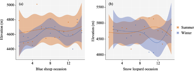
Fig. 3 Seasonal variation in elevations for blue sheep (Pseduois nayaur) and snow leopard (Panthera uncia) in two seasons, winter and summer.

Note: Lines show medians of the posterior distribution, shaded areas show the 95% confidence intervals, and points show each of the 6-day means of the raw data for 90 days of winter (Nov. 2017-Jan. 2018) and summer (May-Jul. 2018).

Even though our results are similar to those reported by Alexander et al. (2016a), we still cannot confirm the relatively poor performing models which contain blue sheep capture index with the winter's negative beta coefficient, most likely due to the uniform distribution of blue sheep across all study areas, although its standard error is large. As such, we caution against any strong interpretations of this parameter and urge further studies to improve the uncalibrated capture indexes as a proxy for density to support a more ideal interpretation (Rovero and Marshall, 2009; Suryawanshi et al., 2013). This issue is particularly important in this region due to the lack of studies on the relationship between snow leopards and their prey.
Our study found that terrain ruggedness (TRI) had distinct seasonal variations in snow leopard habitat use. It showed a strong positive influence in the cold winter, but a much weaker influence during the warm summer. It also showed that TRI affected habitat use on a broad scale (4000 m) in winter but on a much finer scale (30 m) in summer. Terrain ruggedness has been considered a significant factor affecting snow leopard habitat use for many reasons, e.g., shelter, for stealth and ambushing prey, marking habitat, etc. (Jackson and Ahlborn, 1989; Fox et al., 1991; McCarthy et al., 2005; Johansson et al., 2015; Dyldaev et al., 2021). Still, only a few studies have mentioned that snow leopards use habitats with varying terrain ruggedness (Jackson, 1996; Riordan et al., 2016; Atzeni et al., 2020). There is a possibility that snow leopards use less rough terrain in summer because they can rely on tall grasses to hide from prey. In that case, the importance of the brokenness and ruggedness would become less prominent when compared with only bare rock outcroppings during dry and cold periods. We highly recommend more quantitative studies on the seasonal effect of terrain ruggedness variation on snow leopard habitat use.
The influence of elevation was not prominent in our univariate models, although it was reported as highly influential to snow leopard site use in the Qilianshan region in China by Alexander et al. (2016a), and Ladakh in India by Watts et al. (2019). While elevation was not as significant in our models, this may because the very high baseline elevation in our study limited our ability to access the entire landscape. Rovero et al. (2020) also reported that a smaller range in elevation might weaken ties between site use and altitude in the Altai mountains in Mongolia. We recommend that further snow leopard camera-trap studies be conducted across broader altitudinal ranges, at least as much as humanly possible, and cover a range of at least 2000 m. Therefore, to acquire details on snow leopard habitat use in extremely high altitudinal environments, studies using satellite tracking technique are urgently needed in such unique landscapes like the Qomolangma, where the rough and high-altitude range makes some habitats inaccessible.

4.2 High grazing activity in snow leopard habitat

Grazing activities were observed in most of our study areas in both seasons, showing a negative influence on snow leopard habitat use but with seasonal variations. Limited arable land and few locally adapted crops, along with the alpine climate and rough terrain of the study area, mean that livestock husbandry plays a vital role in the local people's lives. Two grazing patterns were observed during the field survey: seasonal and yearly pastures. On the different types of pastures, stony bunkers for herdsmen and livestock had been sparsely built at various elevations. Groups of shepherds (around 5-6 people) with livestock-guarding dogs would spend two months in the mountains looking after a large flock belonging to several families, although they would change to new locations during that time depending on local pasture conditions. A pastoralist accompanied each smaller group of livestock during the day, returning to the sheepcotes before sunset. The importance of herding in the local economy caused the high observation rate for grazing activities in both seasons in our study. The impact of the ANTHROPOGENIC INFLUENCE model was higher than the other summer models, most likely because of more nutritious pastures, leading to more intensive herding activities than in the harsh winter. In addition, the local herding habits can deter predators to some degree, which can explain our observations.

4.3 The difficulty of measuring anthropogenic variables

We tested human settlement and traffic road as anthropogenic variables, using two different measurement methods: Euclidean distance (Dist.) and kernel density (KD). Both of these methods produced unsuitable results. The snow leopard's habitat is in remote mountains with vast wildness and a relatively low human population density. In other words, the immediate (non-climatic) human impact, such as disturbance by even sparsely distributed traffic, settlements, etc., affects the landscape in a fragmented way. However, these influences are usually measured as the straight-line distance between a site and the point of human activities (a road or settlement). This method is used because it is easy to measure quantitatively and to interpret. Nevertheless, variables generated in such a straightforward way may not always accurately represent the situation as perceived by the focal species in a specific environment from within the perspective of landscape ecology. For example, the linear distance to a road can be treated as a potential determinant of the probability of snow leopard site use. However, it only assumes an ideal condition that a species moves on a two-dimensional surface and depicts a line between the site and the center of disturbance to represent the effects but without defining any scope of it. Kernel density may improve matters by delimiting the boundary of the influence, reaching the maximum, and then gradually receding to zero within the radius, which depends on the scale of the disturbance area and the intensity. Nevertheless, it still can be seen as a horizontal vector essentially.
The reasons discussed above may explain why our univariate model containing these covariates did not perform very well. They also might explain why we could repeatedly observe the presence of snow leopards at a site with a short linear distance from a road (dist. 928 m) near the largest and busiest township. This site was at an elevation of 4628 m, while the township was at 4221 m. Incorporating only the ideal two dimensions into measurements could further impair model performance because it simplifies the variables of anthropogenic influence in a real complex landform. Alexander et al. (2016a) also reported finding little empirical support for road distance determining the probability of winter site use by snow leopards in Qilianshan NNR in central China. However, they hypothesized that it could be a potential influencing factor for site use in other seasons with a higher usage rate. In our study, however, we found little empirical evidence for its role in either winter or summer.
Our findings do not necessarily suggest that snow leopards can thrive under such anthropogenic influence. Rather they indicate the risk that inappropriate covariate selection might produce overfitting models, instead of producing models that accurately represent the probability of habitat use, especially given the small sample size due to the challenging terrain and costly surveys. For guiding smarter decisions to benefit both the local ecosystems and rural communities in the future, we encourage more extensive long-term studies, including satellite position tracking for dynamic monitoring of how the growing human activities influence snow leopards and the necessary livelihood development for the local people.

5 ConclusionsAcknowledgments

Snow leopards use their habitat in ways which vary between seasons, and there are complex interactions between covariates. There is realistic complexity in the measurements for some anthropogenic covariates that should be noted when they are incorporated into models. The techniques of landscape ecology applied in snow leopard studies provide a dynamic viewpoint across spatial and temporal scales, improving our understanding of snow leopard habitat use. We speculate that there might still be some important unknown covariates during the summer that affect snow leopard habitat use in this area, which were not observed in this study. The northern side of Mount Qomolangma in QNNR is an extremely high elevation environment that makes field surveys formidable and very expensive, consuming large amounts of time and manpower. Therefore, we strongly recommend the use of an alternative technique such as satellite tracking, which has multiple advantages in such a unique border nature reserve area.
We acknowledge the support from the Snow Leopard Conservation Strategy and Vanke Foundation. We thank the Forestry and Grassland Bureau of Tibet Autonomous Region and the Qomolangma National Nature Reserve Administration. We are also thankful for the support of the fieldwork by CUI Hongyan, YANG Fan from the Eco-Bridge Continental; and Zhala SANGBO, Nyima TANTSENG from the Everest Snow Leopard Conservation Center. Thanks for the technical advice from HUANG Cheng, YANG Li from Sun Yat-sen University; Luciano ATZENI, DENG Zhixiong, WANG Jun, and YU Zibo from Beijing Forestry University, Fudan University, Manchester Metropolitan University, and Beijing Normal University, respectively. Thanks for manuscript advice by Gary Smith from Edinburgh University. We also thank the local residents and officials for their support and insights.

Supplementary tables

Table S1 Chi-square probability (χ2p) and over dispersion statistic c-hat (ĉ) results of the MacKenzie and Bailey (2004) goodness-of-fit (GoF) test for snow leopard (Panthera uncia) habitat use models with different collapsing day-periods
Collapsing scenarios_winter χ²p Collapsing scenarios_summer χ²p
5-day sampling occasions 0.1882 0.4276 5-day sampling occasions 0.0133 7.4845
10-day sampling occasions 0.1414 1.3309 10-day sampling occasions 0.0782 1.9145
15-day sampling occasions 0.2261 1.0823 15-day sampling occasions 0.1551 1.2427
18-day sampling occasions 0.1566 1.2545 18-day sampling occasions 0.2545 1.0112

Note: Detection probability (p) was a binary covariate indicating which of the two survey teams placed a particular camera trap (TEAM). Site use covariates were blue sheep camera-trap capture rates (BS), grazing activity camera trap rates (GRAZE), terrain ruggedness index (TRI) with multiple scales of 30 m, 300 m, 1000 m, 2000 m, and 4000 m (TRI30, TRI300, TRI1000, TRI2000, TRI4000), slopes (SLP) with multi-scales of 30 m, 300 m, 1000 m, 2000 m, 4000 m (SLP30, SLP300, SLP1000, SLP2000, SLP4000). The dataset was limited to 90 sampling days in each season and the effective camera-trap stations numbered 61 and 62 in winter and summer, respectively.

Table S2 Summary of model-averaged parameter estimates of the probability of habitat use (ψ) and detection () for snow leopards (Panthera uncia) at two seasons in Qomolangma NNR
Models_winter ψ±SE ±SE Models_summer ψ±SE ±SE
HABITAT 0.46±0.08 0.18±0.04 A.I. 0.44±0.15 0.18±0.06
TOP. 0.43±0.09 0.19±0.05 TOP. 0.45±0.18 0.18±0.06
GLOBAL 0.46±0.09 0.18±0.04 PREY+A.I. 0.50±0.22 0.16±0.06
TOP. +A.I. 0.43±0.10 0.19±0.05 PREY 0.49±0.17 0.17±0.06
A.I. 0.45±0.13 0.18±0.05 TOP. +A.I. 0.42±0.18 0.19±0.06
PREY 0.46±0.13 0.18±0.05 NULL 0.36±0.10 0.23±0.07
NULL 0.35±0.08 0.24±0.05 HABITAT 0.47±0.20 0.18±0.06
PREY+A.I. 0.46±0.15 0.18±0.06 GLOBAL 0.43±0.20 0.19±0.06
Model averaged 0.44±0.11 0.19±0.05 Model averaged 0.45±0.18 0.19±0.06

Note: Models: TOPOGRAPHY (TOP.), ANTHROPOGENIC INFLUENCE (A.I.); standard error (SE); model-averaged estimates across all models with unconditional standard errors.

Table S3 Correlation matrix of the continuous covariates in winter
Dist._
sett
KD_
sett
Dist._
road
KD_
road
TRI30 TRI300 TRI1000 TRI2000 TRI4000 ELE30 ELE300 ELE1000 ELE2000 ELE4000 BS Graze SLP30 SLP300 SLP1000 SLP2000
KD_sett -0.632
Dist._road 0.233 -0.443
KD_road 0.071 0.188 -0.645
TRI30 -0.064 0.127 -0.141 -0.066
TRI300 -0.186 0.297 -0.126 -0.092 0.441
TRI1000 -0.324 0.372 -0.120 -0.112 0.330 0.657
TRI2000 -0.336 0.305 -0.143 -0.090 0.242 0.436 0.832
TRI4000 -0.148 -0.015 0.091 -0.220 0.216 0.398 0.615 0.775
ELE30 0.549 -0.475 0.385 0.030 -0.263 -0.262 -0.333 -0.321 -0.149
ELE300 0.562 -0.513 0.396 0.027 -0.257 -0.303 -0.359 -0.346 -0.169 0.995
ELE1000 0.615 -0.600 0.413 0.009 -0.233 -0.352 -0.394 -0.402 -0.242 0.944 0.968
ELE2000 0.643 -0.699 0.445 0.000 -0.240 -0.359 -0.420 -0.395 -0.229 0.860 0.892 0.959
ELE4000 0.632 -0.796 0.478 -0.036 -0.164 -0.244 -0.377 -0.342 -0.120 0.746 0.780 0.851 0.940
BS -0.346 0.142 -0.105 -0.153 0.158 0.159 0.336 0.283 0.109 -0.192 -0.190 -0.168 -0.171 -0.154
Graze 0.094 -0.194 0.098 -0.071 0.007 -0.160 -0.067 -0.032 -0.049 0.001 0.026 0.087 0.152 0.157 -0.063
SLP30 -0.172 0.287 -0.259 -0.035 0.911 0.563 0.374 0.318 0.262 -0.385 -0.394 -0.404 -0.425 -0.344 0.181 -0.080
SLP300 -0.151 0.284 -0.178 -0.085 0.326 0.896 0.622 0.438 0.406 -0.213 -0.253 -0.323 -0.335 -0.240 0.137 -0.170 0.443
SLP1000 -0.027 0.142 0.004 -0.220 0.272 0.582 0.691 0.554 0.557 -0.138 -0.160 -0.192 -0.232 -0.187 0.143 -0.171 0.260 0.711
SLP2000 0.072 -0.202 0.234 -0.323 0.262 0.366 0.513 0.500 0.703 -0.052 -0.055 -0.071 -0.048 0.047 0.135 -0.131 0.215 0.468 0.809
SLP4000 0.177 -0.394 0.231 -0.200 0.232 0.236 0.359 0.372 0.623 -0.066 -0.054 -0.061 0.015 0.205 0.023 -0.074 0.164 0.302 0.519 0.831

Note: Pairs of covariates were considered as having high collinearity when |r|>0.6 (values in bold). Site covariates tested were: elevation with five multi-scale 30 m, 300 m, 1000 m, 2000 m, 4000 m threshold values (ELE30, ELE300, ELE1000, ELE2000, ELE4000), slope with five multi-scale threshold values 30 m, 300 m, 1000 m, 2000 m, 4000 m (SLP30, SLP300, SLP1000, SLP2000, SLP4000), terrain ruggedness index with five multi-scale threshold values 30 m, 300 m, 1000 m, 2000 m, 4000 m (TRI30, TRI300, TRI1000, TRI2000,TRI4000), grazing activity index (GRAZE), blue sheep index (BS), kernel density of human settlement (KD_SETT) and road (KD_ROAD), and distance to the human settlement (Dist._SETT) and road (Dist._ROAD).

Table S4 Correlation matrix of the continuous covariates in summer
BS Graze Dist._
SETT
KD_
SETT
Dist._
ROAD
KD_
ROAD
TRI30 TRI300 TRI1000 TRI2000 TRI4000 ELE30 ELE300 ELE1000 ELE2000 ELE4000 SLP30 SLP300 SLP1000 SLP2000
Graze -0.093
Dist._SETT -0.109 -0.126
KD_SETT 0.002 0.051 -0.629
Dist._ROAD -0.018 -0.115 0.290 -0.492
KD_ROAD -0.124 0.140 0.030 0.205 -0.631
TRI30 0.184 0.020 -0.151 0.141 -0.175 -0.072
TRI300 0.332 -0.044 -0.149 0.170 -0.160 -0.062 0.434
TRI1000 0.327 0.012 -0.209 0.161 -0.060 -0.086 0.320 0.670
TRI2000 0.301 0.072 -0.229 0.160 -0.118 -0.039 0.275 0.481 0.865
TRI4000 0.399 0.059 -0.088 -0.058 0.028 -0.125 0.275 0.432 0.665 0.793
ELE30 -0.136 -0.243 0.581 -0.543 0.422 0.005 -0.362 -0.319 -0.245 -0.246 -0.153
ELE300 -0.159 -0.214 0.587 -0.576 0.434 0.001 -0.363 -0.348 -0.256 -0.258 -0.166 0.995
ELE1000 -0.203 -0.150 0.626 -0.649 0.454 -0.018 -0.340 -0.355 -0.253 -0.277 -0.218 0.950 0.971
ELE2000 -0.188 -0.125 0.642 -0.732 0.482 -0.019 -0.347 -0.340 -0.259 -0.273 -0.219 0.874 0.901 0.960
ELE4000 -0.148 -0.124 0.627 -0.818 0.502 -0.042 -0.262 -0.221 -0.198 -0.211 -0.112 0.752 0.782 0.851 0.942
SLP30 0.211 0.023 -0.228 0.312 -0.295 -0.027 0.908 0.548 0.347 0.326 0.300 -0.462 -0.475 -0.480 -0.496 -0.410
SLP300 0.420 -0.036 -0.103 0.158 -0.215 -0.057 0.279 0.871 0.627 0.478 0.439 -0.278 -0.301 -0.316 -0.310 -0.217 0.399
SLP1000 0.413 -0.062 0.023 -0.024 0.026 -0.177 0.191 0.586 0.741 0.649 0.620 -0.115 -0.120 -0.101 -0.129 -0.079 0.189 0.734
SLP2000 0.483 -0.026 0.083 -0.239 0.204 -0.252 0.200 0.438 0.662 0.635 0.733 -0.040 -0.036 -0.020 -0.009 0.073 0.167 0.553 0.884
SLP4000 0.390 -0.018 0.168 -0.372 0.203 -0.158 0.210 0.332 0.565 0.551 0.695 -0.078 -0.064 -0.043 0.025 0.194 0.153 0.409 0.666 0.867

Note: Pairs of covariates were considered as having high collinearity when |r|>0.6 (values in bold). Site covariates tested were: elevation with five multi-scale threshold values 30 m, 300 m, 1000 m, 2000 m, 4000 m (ELE30, ELE300, ELE1000, ELE2000, ELE4000), slope with five multi-scale threshold values 30 m, 300 m, 1000 m, 2000 m, 4000 m (SLP30, SLP300, SLP1000, SLP2000, SLP4000), terrain ruggedness index with five multi-scale threshold values 30 m, 300 m, 1000 m, 2000 m, 4000 m (TRI30, TRI300, TRI1000, TRI2000,TRI4000), grazing activity index (GRAZE), blue sheep index (BS), kernel density of human settelment (KD_SETT) and road (KD_ROAD), and distance to the human settlement (Dist._SETT) and road (Dist._ROAD).

Table S5 Portion of snow leopard (Panthera uncia) single covariate occupancy models (ψ) in winter and summer
Models_winter AICc ∆AICc AICcw Model
Likelihood
K -2 log LL Models_summer AICc ∆AICc AICcw Model
Likelihood
K -2 log LL
ψ(SLP1000) 165.17 0.00 0.9517 1.0000 4 156.46 ψ(SLP1000) 149.41 0.00 0.1154 1.0000 4 140.71
ψ(TRI4000) 173.10 7.93 0.0181 0.0190 4 164.39 ψ(SLP4000) 150.07 0.66 0.0830 0.7189 4 141.37
ψ(TRI1000) 173.17 8.00 0.0174 0.0183 4 164.46 ψ(TRI30) 150.16 0.75 0.0793 0.6873 4 141.46
ψ(SLP300) 176.19 11.02 0.0039 0.0040 4 167.48 ψ(SLP2000) 150.21 0.80 0.0774 0.6703 4 141.51
ψ(SLP2000) 176.49 11.32 0.0033 0.0035 4 167.78 ψ(.) 150.50 1.09 0.0669 0.5798 3 144.09
ψ(TRI2000) 176.67 11.50 0.0030 0.0032 4 167.96 ψ(GRAZE) 150.57 1.16 0.0646 0.5599 4 141.87
ψ(TRI300) 177.94 12.77 0.0016 0.0017 4 169.23 ψ(TRI4000) 150.80 1.39 0.0576 0.4991 4 142.10
ψ(ELE2000) 181.79 16.62 0.0002 0.0002 4 173.08 ψ(SLP300) 150.87 1.46 0.0556 0.4819 4 142.17
ψ(SLP4000) 182.43 17.26 0.0002 0.0002 4 173.72 ψ(SLP30) 150.91 1.50 0.0545 0.4724 4 142.21
ψ(ELE4000) 183.20 18.03 0.0001 0.0001 4 174.49 ψ(TRI1000) 151.47 2.06 0.0412 0.3570 4 142.77
ψ(ELE1000) 183.51 18.34 0.0001 0.0001 4 174.80 ψ(BS) 151.67 2.26 0.0373 0.3230 4 142.97
ψ(KD_SETT) 184.08 18.91 0.0001 0.0001 4 175.37 ψ(TRI300) 152.02 2.61 0.0313 0.2712 4 143.32
ψ(.) 185.15 19.98 0.0000 0.0000 3 178.73 ψ(Dist._SETT) 152.20 2.79 0.0286 0.2478 4 143.50
ψ(ELE300) 185.34 20.17 0.0000 0.0000 4 176.63 ψ(KD_ROAD) 152.41 3.00 0.0258 0.2231 4 143.71
ψ(SLP30) 185.58 20.41 0.0000 0.0000 4 176.87 ψ(TRI2000) 152.43 3.02 0.0255 0.2209 4 143.73
ψ(TRI30) 185.92 20.75 0.0000 0.0000 4 177.21 ψ(Dist._ROAD) 152.52 3.11 0.0244 0.2112 4 143.82
ψ(ELE30) 185.96 20.79 0.0000 0.0000 4 177.25 ψ(ELE2000) 152.64 3.23 0.0230 0.1989 4 143.94
ψ(KD_ROAD) 186.06 20.89 0.0000 0.0000 4 177.35 ψ(ELE4000) 152.71 3.30 0.0222 0.1920 4 144.01
ψ(Dist._SETT) 186.40 21.23 0.0000 0.0000 4 177.69 ψ(ELE30) 152.75 3.34 0.0217 0.1882 4 144.05
ψ(GRAZE) 187.16 21.99 0.0000 0.0000 4 178.45 ψ(ELE300) 152.76 3.35 0.0216 0.1873 4 144.06
ψ(BS) 187.26 22.09 0.0000 0.0000 4 178.55 ψ(KD_SETT) 152.77 3.36 0.0215 0.1864 4 144.07
ψ(Dist._ROAD) 187.37 22.20 0.0000 0.0000 4 178.66 ψ(ELE1000) 152.78 3.37 0.0214 0.1854 4 144.08

Note: Akaike's information criterion corrected for small sample sizes (AICc), relative difference in AICc values compared with the top ranked model (ΔAICc), model weight (AICcw), Model Likelihood, number of parameters (K), and -2log-likelihood (-2 log LL). Detection covariate was camera trap deployment team (TEAM). Site covariates were: elevation with multi-scale threshold values of 30 m, 300 m, 1000 m, 2000 m, 4000 m (ELE30, ELE300, ELE1000, ELE2000, ELE4000), slope with multi-scale threshold values of 30 m, 300 m, 1000 m, 2000 m, 4000 m (SLP30, SLP300, SLP1000, SLP2000, SLP4000), terrain ruggedness index with multi-scale threshold values of 30 m, 300 m, 1000 m, 2000 m, 4000 m (TRI30, TRI300, TRI1000, TRI2000,TRI4000), grazing activity index (GRAZE), blue sheep index (BS), kernel density of human settlement (KD_SETT) and road (KD_ROAD), and distance to the human settlement (Dist._SETT) and road (Dist._ROAD).

Table S6 True optimum multi-scale approach of topographic gradient variables of snow leopard (Panthera uncia) habitat use in winter and summer
Models_winter AICc ∆AICc AICcw Model
Likelihood
K -2 log LL Models_summer AICc ∆AICc AICcw Model
Likelihood
K -2 log LL
ψ(TRI4000+SLP1000) 162.61 0.00 0.7130 1.0000 5 151.52 ψ(.) 150.50 0.00 0.1259 1.0000 3 144.09
ψ(TRI2000+SLP1000) 166.46 3.85 0.1040 0.1459 5 155.37 ψ(TRI30+SLP1000) 150.68 0.18 0.1151 0.9139 5 139.61
ψ(TRI300+SLP1000) 167.09 4.48 0.0759 0.1065 5 156.00 ψ(TRI30+SLP4000) 150.99 0.49 0.0985 0.7827 5 139.92
ψ(TRI30+SLP1000) 167.49 4.88 0.0621 0.0872 5 156.40 ψ(TRI30+SLP2000) 151.34 0.84 0.0827 0.6570 5 140.27
ψ(TRI4000+SLP300) 169.02 6.41 0.0289 0.0406 5 157.93 ψ(TRI300+SLP1000) 151.71 1.21 0.0688 0.5461 5 140.64
ψ(TRI1000+SLP4000) 173.17 10.56 0.0036 0.0051 5 162.08 ψ(TRI30+SLP300) 151.95 1.45 0.0610 0.4843 5 140.88
ψ(TRI300+SLP2000) 173.29 10.68 0.0034 0.0048 5 162.20 ψ(TRI2000+SLP4000) 151.95 1.45 0.0610 0.4843 5 140.88
ψ(TRI2000+SLP300) 174.19 11.58 0.0022 0.0031 5 163.10 ψ(TRI4000+SLP30) 152.05 1.55 0.0580 0.4607 5 140.98
ψ(TRI1000+SLP2000) 174.40 11.79 0.0020 0.0028 5 163.31 ψ(TRI300+SLP4000) 152.39 1.89 0.0489 0.3887 5 141.32
ψ(TRI1000+SLP30) 175.21 12.60 0.0013 0.0018 5 164.12 ψ(TRI4000+SLP300) 152.43 1.93 0.0480 0.3810 5 141.36
ψ(TRI4000+SLP30) 175.30 12.69 0.0013 0.0018 5 164.21 ψ(TRI1000+SLP4000) 152.44 1.94 0.0477 0.3791 5 141.37
ψ(TRI2000+SLP2000) 176.53 13.92 0.0007 0.0009 5 165.44 ψ(TRI300+SLP2000) 152.56 2.06 0.0449 0.3570 5 141.49
ψ(TRI300+SLP4000) 177.22 14.61 0.0005 0.0007 5 166.13 ψ(TRI1000+SLP30) 152.61 2.11 0.0438 0.3482 5 141.54
ψ(TRI30+SLP300) 178.57 15.96 0.0002 0.0003 5 167.48 ψ(TRI2000+SLP300) 153.23 2.73 0.0322 0.2554 5 142.16
ψ(TRI2000+SLP4000) 178.59 15.98 0.0002 0.0003 5 167.50 ψ(TRI2000+SLP30) 153.24 2.74 0.0320 0.2541 5 142.17
ψ(TRI30+SLP2000) 178.86 16.25 0.0002 0.0003 5 167.77 ψ(TRI300+SLP30) 153.27 2.77 0.0315 0.2503 5 142.20
ψ(TRI2000+SLP30) 178.92 16.31 0.0002 0.0003 5 167.83
ψ(TRI300+SLP30) 179.52 16.91 0.0002 0.0002 5 168.43
ψ(TRI30+SLP4000) 184.43 21.82 0.0000 0.0000 5 173.34
ψ(.) 185.15 22.54 0.0000 0.0000 3 178.73

Note: Akaike's information criterion corrected for small sample sizes (AICc), relative difference in AICc values compared with the top ranked model (ΔAICc), model weight (AICcw), Model likelihood, number of parameters (K), and -2log-likelihood (-2 log LL). Detection covariate was camera trap deployment team (TEAM). Site covariates were: elevation with multi-scale threshold values of 30m, 300 m, 1000 m, 2000 m, 4000 m (ELE30, ELE300, ELE1000, ELE2000, ELE4000), slope with multi-scale threshold values of 30 m, 300 m, 1000 m, 2000 m, 4000 m (SLP30, SLP300, SLP1000, SLP2000, SLP4000), terrain ruggedness index with multi-scale threshold values of 30 m, 300 m, 1000 m, 2000 m, 4000 m (TRI30, TRI300, TRI1000, TRI2000,TRI4000).

[1]
Alexander J S, Shi K, Tallents L A, et al. 2016a. On the high trail: Examining determinants of site use by the endangered snow leopard Panthera uncia in Qilianshan, China. Oryx, 50(2): 231-238.

DOI

[2]
Alexander J S, Zhang C C, Shi K, et al. 2016b. A spotlight on snow leopard conservation in China. Integrative Zoology, 11(4): 308-321.

DOI

[3]
Atzeni L, Cushman S A, Bai D F, et al. 2020. Meta-replication, sampling bias, and multi-scale model selection: A case study on snow leopard (Panthera uncia) in western China. Ecology and Evolution, 10(14): 7686-7712.

DOI

[4]
Bai D F, Chen P J, Atzeni L, et al. 2018. Assessment of habitat suitability of the snow leopard (Panthera uncia) in Qomolangma National Nature Reserve based on MaxEnt modeling. Zoological Research, 39(6): 373-386.

[5]
Bailey L L, MacKenzie D I, Nichols J D. 2014. Advances and applications of occupancy models. Methods in Ecology and Evolution, 5(12): 1269-1279.

DOI

[6]
Bailey T N. 1993. The African leopard:Ecology and behavior of a solitary felid. New York, USA: Columbia University Press.

[7]
Barber-Meyer S M, Jnawali S R, Karki J B, et al. 2013. Influence of prey depletion and human disturbance on tiger occupancy in Nepal. Journal of Zoology, 289(1): 10-18.

DOI

[8]
Braczkowski A R, O'Bryan C J, Stringer M J, et al. 2018. Leopards provide public health benefits in Mumbai, India. Frontiers in Ecology and the Environment, 16(3): 176-182.

DOI

[9]
Chamaillé-Jammes S, Valeix M, Bourgarel M, et al. 2009. Seasonal density estimates of common large herbivores in Hwange National Park, Zimbabwe. African Journal of Ecology, 47(4): 804-808.

DOI

[10]
Chen P J, Gao Y F, Lee A T L, et al. 2016. Human-carnivore coexistence in Qomolangma (Mt. Everest) nature reserve, China: Patterns and compensation. Biological Conservation, 197: 18-26.

DOI

[11]
Chen P J, Gao Y F, Wang J, et al. 2017. Status and conservation of the endangered snow leopard Panthera uncia in Qomolangma National Nature Reserve, Tibet. Oryx, 51(4): 590-593.

DOI

[12]
Chen Y S, Liu J P, Wang Z Z. 2013. Dingri County annals. Beijing, China: China Tibetology Press. (in Chinese)

[13]
Cosentino B J, Marsh D M, Jones K S, et al. 2014. Citizen science reveals widespread negative effects of roads on amphibian distributions. Biological Conservation, 180: 31-38.

DOI

[14]
Cushman S A, Gutzweiler K, Evans J S, et al. 2010. The gradient paradigm:A conceptual and analytical framework for landscape ecology. In: Samuel A C, Falk H (eds.). Spatial complexity, informatics, and wildlife conservation. Berlin, Germany: Springer.

[15]
Dias T C, Stabach J A, Huang Q Y, et al. 2020. Habitat selection in natural and human-modified landscapes by capybaras (Hydrochoerus hydrochaeris), an important host for Amblyomma sculptum ticks. Plos One, 15(8): e0229277. DOI: 10.1371/journal.pone.0229277.

DOI

[16]
Dunning J B, Danielson B J, Pulliam H R. 1992. Ecological processes that affect populations in complex landscapes. Oikos, 65(1): 169-175.

DOI

[17]
Dyldaev M, Chymyrov A, Mukabaev A, et al. 2021. Investigation of the population area of snow leopard in the Central Tian-Shan Mountains. E3S Web of Conferences, 227: 02002. DOI: 10.1051/e3sconf/202122702002.

DOI

[18]
Filla M, Lama R P, Ghale T R, et al. 2020. In the shadows of snow leopards and the Himalayas: Density and habitat selection of blue sheep in Manang, Nepal. Ecology and Evolution, 11(1): 108-122.

DOI

[19]
Forrest J L, Wikramanayake E, Shrestha R, et al. 2012. Conservation and climate change: Assessing the vulnerability of snow leopard habitat to treeline shift in the Himalaya. Biological Conservation, 150(1): 129-135.

DOI

[20]
Fox J L, Sinha S P, Chundawat R S, et al. 1991. Status of the snow leopard Panthera uncia in Northwest India. Biological Conservation, 55(3): 283-298.

DOI

[21]
Ghoshal A, Bhatnagar Y V, Pandav B, et al. 2019. Assessing changes in distribution of the Endangered snow leopard Panthera uncia and its wild prey over 2 decades in the Indian Himalaya through interview-based occupancy surveys. Oryx, 53(4): 620-632.

DOI

[22]
Heltai M. 2013. Urban wildlife: Conflict or coexistence? Review on Agriculture and Rural Development, 2(1): 17-23.

[23]
Hilty J A, Kelley A T H, Merenlender W Z, et al. 2019. Corridor ecology:Linking landscapes for biodiversity conservation and climate adaptation. Washington DC, USA: Island Press.

[24]
Hines J E. 2006. PRESENCE2: Software to estimate patch occupancy and related parameters. USGS-PWRC. http://www.Mbr-Pwrc.Usgs.Gov/Software/Presence.html.

[25]
Hines J E, Nichols J D, Royle J A, et al. 2010. Tigers on trails: Occupancy modeling for cluster sampling. Ecological Applications, 20(5): 1456-1466.

DOI

[26]
Huang B. 2019. China statisitical yearbook (township). Beijing, China: China Statistic Press.. (in Chinese)

[27]
Jackson R M, Mallon D, Mishra C, et al. 2014. Snow leopard survival strategy: Revised version 2014. https://www.snowleopardsurvival.org/.

[28]
Jackson R M. 1996. Home range, movements and habitat use of snow leopard (Panthera uncia) in Nepal. Diss., London, UK: University of London.

[29]
Jackson R M, Ahlborn G, 1989. Snow leopards (Panthera uncia) in Nepal-Home range and movements. National Geographic Research, 5: 161-175.

[30]
Jackson R M, Hunter D O. 2003. Snow leopard survey and conservation handbook. https://www.worldcat.org/title/snow-leopard-survey-and-conservation-handbook/oclc/228105447.

[31]
Johansson Ö, Koehler G, Rauset G R, et al. 2018. Sex-specific seasonal variation in Puma and snow leopard home range utilization. Ecosphere, 9(8): e02371. DOI: 10.1002/ecs2.2371.

DOI

[32]
Johansson Ö, McCarthy T, Samelius G, et al. 2015. Snow leopard predation in a livestock dominated landscape in Mongolia. Biological Conservation, 184: 251-258.

DOI

[33]
Johnson D H. 1980. The comparison of usage and availability measurements for evaluating resource preference. Ecology, 61(1): 65-71.

DOI

[34]
Klaassen B, Broekhuis F. 2018. Living on the edge: Multiscale habitat selection by cheetahs in a human-wildlife landscape. Ecology and Evolution, 8(15): 7611-7623.

DOI PMID

[35]
Lewis J S, Logan K A, Alldredge M W, et al. 2015. The effects of urbanization on population density, occupancy, and detection probability of wild felids. Ecological Applications, 25(7): 1880-1895.

DOI

[36]
Li J, McCarthy T M, Wang H, et al. 2016. Climate refugia of snow leopards in high Asia. Biological Conservation, 203: 188-196.

DOI

[37]
Li J, Wang D J, Yin H, et al. 2014. Role of Tibetan buddhist monasteries in snow leopard conservation. Conservation Biology, 28(1): 87-94.

DOI

[38]
Li J, Weckworth B V, McCarthy T M, et al. 2020. Defining priorities for global snow leopard conservation landscapes. Biological Conservation, 241: 108387. DOI: 10.1016/j.biocon.2019.108387.

DOI

[39]
Long R A, Donovan T M, MacKay P, et al. 2011. Predicting carnivore occurrence with noninvasive surveys and occupancy modeling. Landscape Ecology, 26(3): 327-340.

DOI

[40]
MacKenzie D I, Bailey L L. 2004. Assessing the fit of site-occupancy models. Journal of Agricultural, Biological, and Environmental Statistics, 9(3): 300-318.

[41]
MacKenzie D I, Nichols J D, Lachman G B, et al. 2002. Estimating site occupancy rates when detection probabilities are less than one. Ecology, 83(8): 2248-2255.

DOI

[42]
MacKenzie D I, Nichols J D, Royle J A, et al. 2006. Occupancy estimation and modeling:Inferring patterns and dynamics of species occurrence. London, UK: Academic Press.

[43]
McCarthy T, Mallon D, Sanderson E W, et al. 2016. What is a snow leopard? Biogeography and status overview. Amsterdam, Netherlands: Elsevier.

[44]
McCarthy T M. 2000. Ecology and conservation of snow leopards, Gobi brown bears, and wild Bactrian camels in Mongolia. Diss., Amherst, USA: University of Massachusetts Amherst.

[45]
McCarthy T M, Chapron G. 2003. Snow leopard survival strategy. Seattle, USA: ISLET and SLN.

[46]
McCarthy T M, Fuller T K, Munkhtsog B. 2005. Movements and activities of snow leopards in Southwestern Mongolia. Biological Conservation, 124(4): 527-537.

DOI

[47]
McGarigal K, Wan H Y, Zeller K A, et al. 2016. Multi-scale habitat selection modeling: A review and outlook. Landscape Ecology, 31(6): 1161-1175.

DOI

[48]
Miehe G, Miehe S, Böhner J, et al. 2014. How old is the human footprint in the world's largest alpine ecosystem? A review of multiproxy records from the Tibetan Plateau from the ecologists' viewpoint. Quaternary Science Reviews, 86: 190-209.

DOI

[49]
Mishra C, Redpath S R, Suryawanshi K R. 2016. Livestock predation by snow leopards:Conflicts and the search for solutions. In: PhiliP J (ed.). Snow leopards. Amsterdam, Netherlands: Elsevier.

[50]
Mobæk R, Mysterud A, Egil Loe L, et al. 2009. Density dependent and temporal variability in habitat selection by a large herbivore: An experimental approach. Oikos, 118(2): 209-218.

DOI

[51]
Nyhus P J, McCarthy T M, Mallon D. 2016. Snow leopards: Biodiversity of the world:Conservation from genes to landscapes. London, UK: Academic Press.

[52]
Oli M K. 1996. Seasonal patterns in habitat use of blue sheep Pseudois nayaur (Artiodactyla, Bovidae) in Nepal. Mammalia, 60(2): 187-194.

[53]
Packer C, Ikanda D, Kissui B, et al. 2005. Lion attacks on humans in Tanzania. Nature, 436(7053): 927-928.

DOI

[54]
Pandit M K, Manish K, Koh L P. 2014. Dancing on the roof of the world: Ecological transformation of the Himalayan landscape. BioScience, 64(11): 980-992.

DOI

[55]
Riordan P, Cushman S A, Mallon D, et al. 2016. Predicting global population connectivity and targeting conservation action for snow leopard across its range. Ecography, 39(5): 419-426.

DOI

[56]
Roberts T J. 1977. The mammals of Pakistan (1st Edition). Kent, UK: Ernest Benn.

[57]
Robinson H S, Weckworth B. 2016. Landscape ecology:Linking landscape metrics to ecological processes. In: Nyhus P J (ed.). Snow leopards: Biodiversity of the world: Conservation from genes to landscapes. London, UK: Elsevier.

[58]
Rovero F, Augugliaro C, Havmøller R W, et al. 2020. Co-occurrence of snow leopard Panthera uncia, Siberian ibex Capra sibirica and livestock: Potential relationships and effects. Oryx, 54(1): 118-124.

DOI

[59]
Rovero F, Marshall A R. 2009. Camera trapping photographic rate as an index of density in forest ungulates. Journal of Applied Ecology, 46(5): 1011-1017.

DOI

[60]
Sarmento W M, Reading R P. 2016. Conservation presence, not socioeconomics, leads to differences in pastoralist perceived threats to argali. Journal of Asia-Pacific Biodiversity, 9(3): 263-270.

DOI

[61]
Schaller G B. 1977. Mountain monarchs:Wild sheep and goats of the Himalaya. Chicago, USA: University of Chicago Press.

[62]
Schaller G B. 1998. Wildlife of the Tibetan steppe. Chicago, USA: University of Chicago Press.

[63]
Sharma R K, Bhatnagar Y V, Mishra C. 2015. Does livestock benefit or harm snow leopards? Biological Conservation, 190: 8-13.

DOI

[64]
Singh E, Rawat N S, Burfal R, et al. 2019. The ancient ceramic tradition of the trans-himalayan region of Spiti Valley, Himachal Pradesh: Based on new findings. Journal of Multidisciplinary Studies in Archaeology, 7: 324-339.

[65]
Snow Leopard China. 2019. Status of snow leopard survey and conservation, China 2018. https://max.book118.com/html/2020/0308/5312013103002230.shtm. in Chinese)

[66]
Snow Leopard Working Secretariat. 2013. Global snow leopard and ecosystem protection program. Bishkek, Kyrgyz Republic: Snow Leopard Working Secretariat.

[67]
Strampelli P, Andresen L, Everatt K T, et al. 2018. Habitat use responses of the African leopard in a human-disturbed region of rural Mozambique. Mammalian Biology, 89: 14-20.

DOI

[68]
Sullivan C D, Chen P J, Alexander J S, et al. 2018. Conflict on the range: Evaluating driving factors of attitudes toward prey species in Qilianshan. Journal of Resources and Ecology, 9(5): 554-565.

DOI

[69]
Sunarto S, Kelly M J, Parakkasi K, et al. 2012. Tigers need cover: Multi-scale occupancy study of the Big Cat in Sumatran Forest and plantation landscapes, Plos One, 7(1): e30859. DOI: 10.1371/journal.pone.0030859.

DOI

[70]
Sunquist M E. 1981. The social organization of tigers (Panthera tigris) in Royal Chitawan National Park, Nepal. Washington, USA: Smithsonian Institution Press.

[71]
Sunquist M E, Sunquist F. 2001. Changing landscapes:Consequences for carnivores. In: Gittleman J L, Funk S M, MacDonald D W, et al. (eds.). Carnivore conservation. Cambridge, UK: Press Syndicate of the University of Cambridge.

[72]
Suryawanshi K R, Bhatia S, Bhatnagar Y V, et al. 2014. Multiscale factors affecting human attitudes toward snow leopards and wolves. Conservation Biology, 28(6): 1657-1666.

DOI

[73]
Suryawanshi K R, Bhatnagar Y V, Redpath S, et al. 2013. People, predators and perceptions: Patterns of livestock depredation by snow leopards and wolves. Journal of Applied Ecology, 50(3): 550-560.

DOI

[74]
Tan C K W, Rocha D G, Clements G R, et al. 2017. Habitat use and predicted range for the mainland clouded leopard Neofelis nebulosa in Peninsular Malaysia. Biological Conservation, 206: 65-74.

DOI

[75]
Taubmann J, Sharma K, Uulu K Z, et al. 2016. Status assessment of the endangered snow leopard Panthera uncia and other large mammals in the Kyrgyz Alay, using community knowledge corrected for imperfect detection. Oryx, 50(2): 220-230.

DOI

[76]
Treves A, Karanth K U. 2003. Human-carnivore conflict and perspectives on carnivore management worldwide. Conservation Biology, 17(6): 1491-1499.

DOI

[77]
Watts S M, McCarthy T M, Namgail T. 2019. Modelling potential habitat for snow leopards (Panthera uncia) in Ladakh, India. Plos One, 14(1): e0211509. DOI: 10.1371/journal.pone.0211509.

DOI

[78]
Wu J G. 2007. Scale and scaling:A cross-disciplinary perspective. In: Wu J G, Hobbs R J (eds.). Key topics in landscape ecology. West Nyack, USA: Cambridge University Press.

[79]
Yirga G, Ersino W, De Iongh H H, et al. 2013. Spotted hyena (Crocuta crocuta) coexisting at high density with people in Wukro District, northern Ethiopia. Mammalian Biology, 78(3): 193-197.

DOI

[80]
Wang Z Z, Wang A Z, Liu W Q. 2013. Dingri County annals. Beijing, China: China Tibetology Press.. (in Chinese)

Outlines

/