Land Use and Sustainable Development

Spatial Patterns of Soil Organic Matter, Nitrogen, Phosphorus and Potassium in a Subtropical Forest and Its Implication for Forest Management

  • HAN Lili , 1 ,
  • LU Yuanchang 2 ,
  • MA Wu 3 ,
  • MENG Jinghui , 1, *
Expand
  • 1. Research Center of Forest Management Engineering of National Forestry and Grassland Administration, Beijing Forestry University, Beijing 100083, China
  • 2. Institute of Forest Resource and Information Techniques, Chinese Academy of Forestry, Beijing 100091, China
  • 3. Department of Forestry and Natural Resources, Purdue University, West Lafayette, Indiana 47906, USA

HAN Lili, E-mail:

Received date: 2020-10-20

  Accepted date: 2021-09-08

  Online published: 2022-04-18

Supported by

The National Key Research & Development Program of China(2016YFD060020501)

Abstract

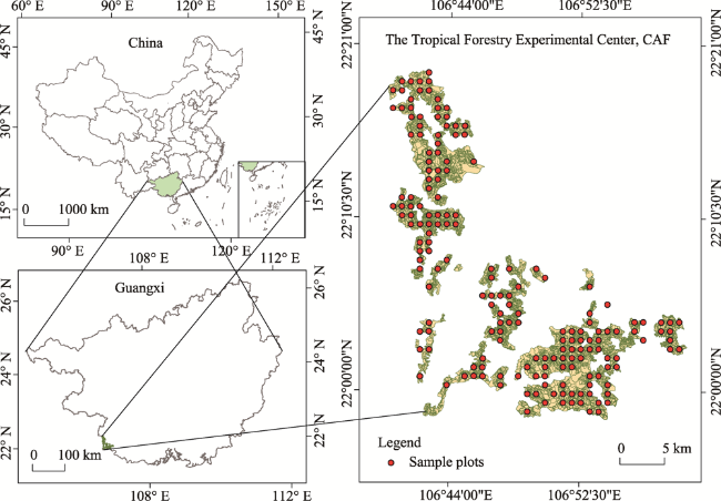
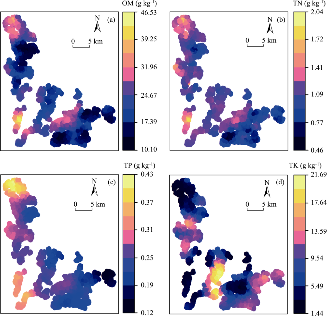
Total nitrogen (TN), total phosphorus (TP), total potassium (TK), and soil organic matter (OM) can significantly affect forest growth. However, these soil properties are spatially heterogeneously distributed, complicating the prescription of forest management strategies. Thus, it is imperative to obtain an in-depth understanding of the spatial distribution of soil properties. In this study, soils were sampled at 181 locations in the Tropical Forest Research Center in the southwestern Guangxi Zhuang Autonomous Region in southern China. We investigated the spatial variability of soil OM, TN, TP, and TK using geostatistical analysis. The nugget to sill ratio indicated a strong spatial dependence of soil TN and a moderate spatial dependence of soil OM, TP, and TK, suggesting that TN was primarily controlled by intrinsic factors (e.g., soil texture, parent material, vegetation type, and topography), whereas soil OM, TP, and TK were controlled by intrinsic and extrinsic factors (e.g., cultivation practices, fertilization, and planting systems). Based on the spatial variability determined by the geostatistical analysis, we performed ordinary kriging to create thematic maps of soil TN, TP, TK, and OM. Model validation indicated that the thematic maps were reliable to inform forest management.

Cite this article

HAN Lili , LU Yuanchang , MA Wu , MENG Jinghui . Spatial Patterns of Soil Organic Matter, Nitrogen, Phosphorus and Potassium in a Subtropical Forest and Its Implication for Forest Management[J]. Journal of Resources and Ecology, 2022 , 13(3) : 417 -427 . DOI: 10.5814/j.issn.1674-764x.2022.03.007

1 Introduction

Owing to its significant influence on the rate of photosynthesis and site productivity, forest soil is considered the most fundamental factor that regulates forest ecological processes and ultimately determines forest structure (Becker et al., 2017; Zavišić et al., 2018). Therefore, the properties of forest soil have been widely explored in forestry to assess the ability of the soil to provide sufficient nutrients for tree growth and stand development. Total nitrogen (TN), total phosphorus (TP), and total potassium (TK) in soil are the primary macronutrients influencing forest growth (Li et al., 2016; Tang et al., 2016; Gao et al., 2019), which are extensively studied to provide valuable information for forest management. For instance, Wright et al. (2011) reported that in the lowland tropics, deficiency in TN, TP, and TK limited the growth of forest plants on relatively fertile soil, and TK was the most limiting nutrient in seedlings, saplings, and poles (1-10 cm in diameter at breast height). In addition to TN, TP, and TK, forest plant growth is also significantly affected by soil organic matter (OM), which provides mineral elements required by plants (Wander, 2004). OM has the largest influence on soil quality and fertility (Reeves, 1997; Franzluebbers, 2002). Additionally, soil TN, TP, TK, and OM are closely linked to environmental problems (Ju et al., 2007; Wang et al., 2009a), biogeochemical cycles (Bronson et al., 2004), greenhouse gas emissions, and global climate change (Merino et al., 2004; Bhattacharyya et al., 2013).
Forest soil properties, e.g., soil TN, TP, TK, and OM in the present study, are determined by biotope conditions and can change over time due to normal processes, such as succession (Wang et al., 2011) and biomass accumulation (Lawrence, 2005). Moreover, soil properties are also significantly influenced by the fertilization of forest land (Knoepp and Swank, 1997; Block et al., 2002; Zhang et al., 2018). The most common example is the use of N, P, and K fertilizers to increase tree or forest growth (Melo et al., 2015). Additionally, many authors documented that various forest management activities, e.g., thinning (Thibodeau et al., 2000; Grady and Hart, 2006), harvesting (Bock and Van Rees, 2002; Kaarakka et al., 2014), and site preparation (Archibold et al., 2000), affect soil properties. For instance, Knoepp and Swank (1997) documented that commercial tree harvesting resulted in substantial increases in the concentrations of C and N in the soil surface following harvesting. Block et al. (2002) reported that soil bulk density increased significantly from preharvest to postharvest. Furthermore, differences in the topography, climatic conditions, vegetation types, and parent materials contribute to the complexity of soil properties and exhibit significant spatial and temporal variability (Wang et al., 2009b; Fu et al., 2014; Tang et al., 2016). The high heterogeneity of the forest soil properties complicates science-based forest soil management; thus, the spatial distribution of soil properties has to be ascertained for sustainable forest management.
Geostatistical technique is a suitable approach to quantify spatial variation of geographical objects (Bohling, 2005) and has been extensively used to estimate the spatial distribution of soil properties (Reza et al., 2017; Bhunia et al., 2018; Zarlenga et al., 2018; Orton et al., 2020). Additionally, geostatistical techniques were also used in other forestry applications, e.g., for the prediction of forest biomass (Sales et al., 2007; Du et al., 2010; Yadav and Nandy, 2015), stem size and increment (Biondi et al., 1994), leaf area index (Berterretche et al., 2005), and forest growing stock (Akhavan, 2010). Geostatistical techniques for spatial interpolation include inverse distance weighting, spline methods, ordinary kriging (OK), co-kriging, simple kriging, and universal kriging (Zimmerman et al., 1999; Schloeder et al., 2001; Meng et al., 2013; Liu et al., 2019). Among the various methods, OK involves a straightforward implementation and is simpler and easier to perform than other kriging approaches. One such approach is co-kriging, which requires covariance modeling, increasing the workload (Tang et al., 2017; Liu et al., 2019). OK has been therefore extensively employed for the estimation of the spatial distribution of soil properties (Arslan, 2012; Dai et al., 2014; Elbasiouny et al., 2014; Tang et al., 2016).
In China, the forest management unit (FMU) serves as the basic unit for conducting forest management activities (Lei et al., 2009). The forest management plan of the FMU is of great importance to sustainable forest management since it defines forest management activities for the next ten years (Wang, 2006). Therefore, it is important to formulate a solid forest management plan. The high heterogeneity of forest soil properties in FMU hinders the prescription of a solid forest management plan and in-depth knowledge of the spatial distribution of soil properties, particularly TN, TP, TK, and OM. These properties are necessary for the development of a forest management plan. The objectives were therefore to: 1) Predict the spatial variability of soil TN, TP, TK, and OM in the FMU using the OK interpolation approach; 2) Produce thematic maps of soil TN, TP, TK, and OM in the FMU.

2 Materials and methods

2.1 Study area

We selected the Tropical Forestry Experimental Center (TFEC) of the Chinese Academy of Forestry as the study area (Fig. 1). The center is located in Pingxiang City in the south of Guangxi Zhuang Autonomous Region (106°41°- 106°59°E, 21°57°-22°16°N) and covers an area of 1.9×10⁵ ha, with a total stocking of 1.39 million m3. The area has a semi-humid and humid monsoon climate with a minimum temperature of 13 ℃ and a maximum temperature of 28 ℃. The average annual sunshine hours are 1614 h, and the annual rainfall is 1062-1772 mm. The elevation ranges from 250 m to 800 m above sea level. The dominant soils are lateritic mountain soil and purple soil. The dominant species/vegetation types are Pinus massoniana, Cunninghamia lanceolata, and mixed broad-leaved plantation (Meng et al., 2014).
Fig. 1 Distribution of the 181 systematic sample plots in the study area

2.2 Data

A total of 181 cluster sample plots were systematically deployed on the basis of a 1 km×1 km grid in the TFEC (Fig. 1). The cluster plots consisted of three circular subplots (radius of 6.51 m), resulting in a total area of the cluster sample plot of 400 m2. Each circular subplot was located 8.49 m from the cluster plot center and was distributed radially in a 0°, 120° and 240° direction, respectively. In each circular subplot, we measured the diameter at breast height (DBH) and the tree height (H). We identified the species of all trees. In each circular subplot center, the soil was sampled down to 60 cm and classified into the following horizons: 0-20 cm, 20-40 cm, and 40-60 cm. In the field, the soil samples from the same sample horizons of the three subplots were mixed to represent the sample of the cluster plot. The soil samples were analyzed in the laboratory, and the soil TN, TP, TK, and OM were derived following the national standard protocol of China (State Forestry Adiministration, 1999). The soil TN, TP, TK, and OM were averaged for the three soil horizons for geostatistical analysis.

2.3 Statistical and geostatistical analysis

We obtained descriptive statistics of the soil TN, TP, TK, and OM from the 181 sample plots (mean, standard deviation, minimum, maximum, P-value of S-W). Because geostatistical analysis requires a normal distribution of data (Rodríguez et al., 2009; Tang et al., 2016; Teng et al., 2017), the Shapiro-Wilk test was performed at the 0.05 significance level to determine normality (Fu et al., 2014; Bhunia et al., 2018). If a non-normal distribution was detected, the data were log-transformed before geostatistical analysis (Rodríguez et al., 2009; Teng et al., 2017).
We used the data to derive the experimental semivariogram to determine the spatial autocorrelation of soil TN, TP, TK, and OM and the range of spatial dependence. The experimental semivariogram was calculated as follows (Fu et al., 2014):
$\gamma (h)=\frac{1}{2N(h)}\sum\limits_{i=1}^{N(h)}{{{[z({{x}_{i}})-z({{x}_{i+h}})]}^{2}}}$
where z(xi) and z(xi+h) denote the values of z at the locations xi and xi+h, xi and xi+h is the locations of i and i+h, h is the lag, γ(h) is the estimate of the semi-variance for lag h and N(h) is the number of pairs of sample points separated by h.
We fitted the semivariogram using four widely used theoretical models, i.e., linear, spherical, Gaussian, and exponential models (Wang et al., 2009b; Tang et al., 2016; Teng et al., 2017). The model with the largest coefficient of determination (R2) and the smallest residual sum of squares (RSS) was considered the best fit model (Wang et al., 2009b; Liu et al., 2013a). The best fit model was used to provide the spatial autocorrelation for the OK spatial interpolation because the weights are determined based on the autocorrelation to ensure an unbiased error and low variance (Liu et al., 2013a).
The nugget (C0), spatial range (A0), and sill (C+C0) are the most important spatial information obtained from the best fit model and provide details on the spatial structure of soil TN, TP, TK, and OM at a particular scale. The total variance (C+C0) represents the sum of the nugget effect (C0, which is the unexplained variability due to measurement error or spatial variability that is undetectable at a given scale) and the structural variance (C, which is the variance accounted for by spatial autocorrelation). A0 indicates the minimum distance beyond which the measured data show no spatial dependence. In addition to the three primary parameters, the C0 to C+C0 ratio is commonly calculated to determine the magnitude of spatial dependence (Liu et al., 2013a; Martín et al., 2016).
We used OK to determine the spatial variability of soil TN, TP, TK, and OM in the 0-60 cm soil horizon and created the thematic maps. R(x), which is the most likely value of a given grid cell for m nearby observations was defined as (Martín et al., 2016; Tang et al., 2016):
$R(x)=\sum\limits_{j=1}^{m}{\mathop{\delta }_{j}}z({{x}_{i}})$
where m is number of locations where measurements are made, z(xi) is the value of z at the location xi and represents the optimal weight with $\sum\limits_{j=1}^{m}{{{\delta }_{j}}=1}$.
All geostatistical analyses were performed using R3.5.1, using the R packages “geoR” and “gstat”, and we produced the thematic maps for TFEC using the R Package “sp”.

2.4 Model validation

We used the leave-one-out cross-validation method (Aelion et al., 2009; Du et al., 2009; Stevens et al., 2012) to evaluate the prediction accuracy of soil TN, TP, TK, and OM. In this approach, we excluded one datum and retained the remaining data for kriging interpolation to provide the predicted value of the excluded datum. We compared the estimated value with the real value of the excluded datum. This process was performed for all observations. The lack-of-fit statistics absolute mean error (AME), mean error (ME), root mean square error (RMSE), and determination coefficient (R2) (Liu et al., 2013a; Liu et al., 2013b), were calculated to evaluate the predictive performance of the OK spatial interpolation:
$AME=\frac{1}{n}\sum\limits_{i=1}^{n}{\left| \mathop{P}_{_{i}}-{{M}_{i}} \right|}$
$ME=\frac{1}{n}\sum\limits_{i=1}^{n}{({{P}_{i}}-{{M}_{i}})}$
$RMSE=\sqrt{\frac{1}{n}\sum\limits_{i=1}^{n}{{{({{P}_{i}}-{{M}_{i}})}^{2}}}}$
$\mathop{R}^{2}=1-\frac{\sum\limits_{i=1}^{n}{{{({{P}_{i}}-{{M}_{i}})}^{2}}}}{\sum\limits_{i=1}^{n}{{{({{M}_{i}}-\bar{M})}^{2}}}}$
where Pi, Mi,$\bar{M}$ and n are the predicted values, measured values, mean values of the measured data, and the number of measured values, respectively.

3 Results and discussion

3.1 Descriptive statistics

The descriptive statistics of soil TN, TP, TK, and OM in the 0-60 cm soil horizon are listed in Table 1. OM ranged from 6.61 g kg-1 to 58.25 g kg-1, with an average of 21.66 g kg-1; this value was lower than the mean value of 45.45 g kg-1 for natural vegetation in China (Li et al., 2013). The low value is attributed to the single-species plantation as the primary vegetation type in the study area, representing 80% of the total forest area. The other 20% was a mixed-species broadleaved forest. Previous studies (Zhang et al., 2005; Forrester et al., 2013) reported that the OM was lower in single-species plantations than mixed-species broadleaved forests, especially conifer plantations. The reason for the higher OM in mixed-species broadleaved forests might be that species diversity accelerates leaf litter decomposition (Taylor et al., 2007). Furthermore, Wang et al., (2007) found that changes in land-use from native broadleaved forest to coniferous plantation reduced the quantity and quality of soil OM.
Table 1 Descriptive statistics of soil TN, TP, TK, and OM in the 0-60 cm soil horizon. (Unit: g kg-1)
Nutrient Mean Min Max Median SD CV (%) P-value of S-W
OM 21.66 6.61 58.25 20.05 9.23 42.62 <0.0001
TN 1.10 0.35 2.50 1.09 0.36 32.75 <0.0001
TP 0.26 0.10 0.74 0.24 0.10 39.04 <0.0001
TK 9.78 0.61 38.03 9.58 7.27 74.38 <0.0001

Note: Min: Minimum value; Max: Maximum value; SD: Standard deviation; CV: Coefficient of variance; S-W test: Shapiro-Wilk test; OM: Organic matter density; TN: Total nitrogen density; TP: Total phosphorus density; TK: Total potassium density.

TN ranged from 0.35 g kg-1 to 2.5 g kg-1, with an average of 1.10 g kg-1. A similar TN value (1.12 g kg-1) was observed by Gao et al. (2019) in the Sichuan Basin in southern China. The values in our study were very close to the mean TN value (1.54 g kg-1) in China (Zhang et al., 2005; Wang et al., 2013). Although the TN value in this study was in the range of 1.0-49.9 Mg ha-1 for N in various forest stands in China (Yang et al., 2007; Tang et al., 2016), the value was substantially lower than that reported in other studies (Tang et al., 2016). The TP range was 0.10-0.74 g kg-1 (average of 0.26 g kg-1), which was lower than the average (0.74 g kg-1) in China (Zhang et al., 2005; Wang et al., 2013). Tang et al. (2016) also reported a value (0.38 g kg-1) lower than the average value in subtropical China. Similarly, TK increased from a minimum of 0.61 g kg-1 to a maximum of 38.03 g kg-1 (average of 9.78 g kg-1), which was close to the value (9.64 g kg-1) reported by Gao et al. (2019). However, these TK values were lower than the mean (18.60 g kg-1) in China (Zhang et al., 2005). In general, our results indicated that soil TN, TP, and TK were lower than the mean values in China, which might be attributed to a lack of fertilization and the removal of TN, TP, and TK due to the extensive timber harvest in the study area (Tang et al., 2016).
In previous studies, coefficients of variance (CV) of 10%, 10%-90%, and >90% were used to indicate low, moderate, and high variability (Liu et al., 2013a; Tang et al., 2016). In our study, the CV ranged from 32.75% to 74.38%, suggesting moderate variability of the soil nutrients. The Shapiro- Wilk test indicated a non-normal distribution of the OM, TN, TP, and TK (P<0.0001) (Table 1). Therefore, a natural logarithmic transformation was used to satisfy the assumption of normality before performing spatial interpolation (Liu et al., 2013a; Tang et al., 2016).

3.2 Spatial distributions of soil OM, TN, TP, and TK

The semivariograms are shown in Fig. 2, and the corresponding parameters are listed in Table 2. The semivariograms of OM, TN, TP, and TK were successfully fitted using the candidate models. The exponential model was the best fit model for TN and TK, whereas the spherical model performed best for OM and TK. The R2 ranged from 0.655 to 0.948, indicating a good fit of the spatial structures of the four soil nutrients for the different semivariogram models. Similar results were also reported by many studies (Tang et al., 2016; Gao et al., 2019). For instance, Tang et al. (2016) found that the exponential model provided the best fit for TN and TP, and the spherical model was the best fit for TK (range of 0.64-0.74 for R2); these results agreed with our results.
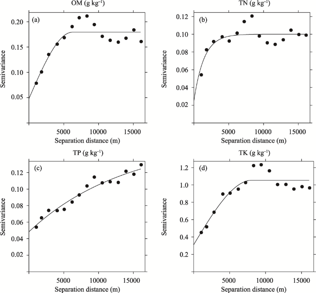
Fig. 2 Experimental semivariograms of soil OM (a), TN (b), TP (c) and TK (d).
Table 2 Models and fitted parameters of the semivariograms of soil OM, TN, TP, and TK. (Unit: g kg-1)
Nutrient Models Nugget (C0) Sill (C0+C) Nugget/Sill Range (A0, m) Determination coefficient
OM Spherical 0.0480 0.1794 0.27 6250 0.815
TN Exponential 0.0250 0.1001 0.25 4347 0.655
TP Exponential 0.0483 0.1598 0.30 14015 0.948
TK Spherical 0.3098 1.0546 0.29 8114 0.848
In this study, the C0 values were lowest for soil TN (0.0250) and highest for soil TK (0.3098). Positive values indicate random and inherent variability or sampling errors (Wang et al., 2009b). The C+C0 values represent the total spatial variation; these values ranged from 0.1001 for TN to 1.0546 for TK.
The C0/(C+C0) ratio indicates spatial dependence (Liu et al., 2013a; Martín et al., 2016; Gao et al., 2019). Ratios of < 25%, 25%-75%, and >75% indicate strong, moderate, and weak spatial dependence, respectively (Cambardella et al., 1994; Tang et al., 2017). In this study, the C0/(C+C0) ratio was 0.25 for TN, demonstrating strong spatial dependence. A similar result for TN was reported by Tang et al. (2016), who analyzed the spatial distribution of soil TN, TP, and TK in Moso Bamboo Forests in Subtropical China. Many authors (Wang et al., 2009b; Fu et al., 2014; Tang et al., 2016) have argued that a strong spatial dependence is the result of soil intrinsic properties (soil texture, parent material, vegetation, and topography), whereas weak spatial dependence is commonly attributed to extrinsic properties (cultivation practices, fertilization, and planting systems, which reduce the spatial correlation of soil nutrients and result in homogenization (Cambardella et al., 1994; Wang et al., 2009b). Thus, the C0/(C+C0) ratio of soil TN was very close to the threshold value (0.25) of strong spatial dependence, suggesting that the intrinsic factors had a larger influence on the spatial patterns than the extrinsic factors. The C0/(C+C0) ratios of OM, TP, and TK were 0.27, 0.29, and 0.30, respectively, indicating moderate spatial dependence. Similar results were also documented by Tang et al. (2016), who attributed the moderate spatial dependence to extrinsic and intrinsic factors. At the TFEC, few fertilization treatments were applied, and the large range in elevation (250-800 m) might have contributed to the moderate spatial dependence. Tang et al. (2016) also concluded that in addition to intensive fertilization and weeding, the large range in elevation might have contributed to the moderate spatial dependence of soil TP and TK in their study.
A0 is the minimum distance beyond which the data show no spatial dependence, whereas, within the spatial range, the data are spatially dependent (Martín et al., 2016; Tang et al., 2016). The smallest A0 was observed for soil TN (4347 m) and the largest for soil TP (14015 m), suggesting that soil TN was the nutrient with the most heterogeneous distribution, and soil TP exhibited high homogeneity. A similar pattern was also reported by Tang et al. (2017) and Liu et al. (2013a). Additionally, it is noteworthy that the values of A0 were generally larger than the sampling interval (1000 m), indicating that the systematic sampling system (1km×1 km) was suitable for examining the spatial patterns of soil TN, TP, TK, and OM in the TFEC (Garten Jr et al., 2007; Liu et al., 2013a; Tang et al., 2016).

3.3 Model validation of OK

We plotted the predicted values versus the measured values to investigate the OK interpolation performance (Fig. 3).Simple linear models were created for the soil properties and were compared with the 1:1 line. We observed that the linear models intersected the 1:1 line. Prior to the intersection, the linear model overestimated the soil properties, whereas, after the intersection, the opposite pattern was detected. Therefore, interpolation showed a centralization effect. This pattern was similar to that observed by other authors who used OK for spatial interpolation (Liu et al., 2013a; Liu et al., 2013b; Tang et al., 2016). Yamamoto (2005) reported that overestimation/underestimation is commonly observed and is due to the smoothing effect of the OK and other interpolation methods based on the weighted average.
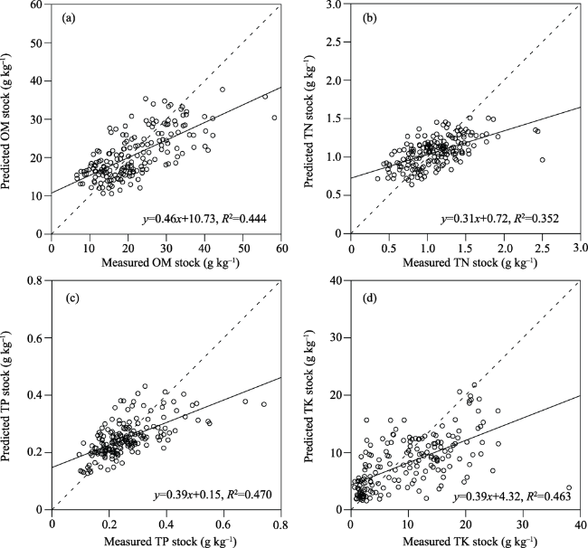
Fig. 3 Cross-validation of kriging interpolation for OM (a), TN (b), TP (c) and TK(d) (dashed line denotes the 1:1 line).
Table 3 shows the cross-validated lack-of-fit statistics (AME, ME, and RMSE). The closer the values are to zero, the better the model performance is. The ME of soil OM, TN, TP, and TK ranged from 0.0017 to 0.0127, demonstrating that OK interpolation resulted in relatively unbiased values. The RMSE, which represents the precision of the spatial interpolation and the error of the spatial interpolation prediction of the sample points, ranged from 0.2626 for soil TP to 0.7192 for soil TK, indicating that soil TP had the highest estimation precision and soil TK had the lowest one.
Table 3 The lack-of-fit statistics of the semivariogram model of soil OM, TN, TP, and TK. (Unit: g kg-1)
Nutrient AME ME RMSE
OM 0.2615 0.0017 0.3185
TN 0.2132 0.0028 0.2704
TP 0.2082 0.0002 0.2626
TK 0.5645 0.0127 0.7192

Note: AME: Absolute mean error; ME: Mean error; RMSE: Root mean square error.

It was noteworthy that the cross-validated R2 ranged from 0.3520 to 0.4695, which was relatively low. However, the R2 values were similar to those of other studies (Fu et al., 2014; Veronesi et al., 2014; Tang et al., 2016). For instance, Tang et al. (2016) reported cross-validated R2 value ranging from 0.37 to 0.47 for the use of OK to determine the spatial distribution of soil TN, TP, and TK. The low R2 might be attributed to the large variability of soil TN, TP, and TK resulting from differences in environmental conditions (Tang et al., 2016).

3.4 Thematic maps and its contribution to forest management

Figure 4 shows the thematic maps of the spatial distributions of soil OM, TN, TP, and TK obtained by OK. The predicted soil OM, TN, TP, and TK ranged from 10.10 g kg-1 to 46.53 g kg-1, 0.46 g kg-1 to 2.04 g kg-1, 0.12 g kg-1 to 0.43 g kg-1, and 1.44 g kg-1 to 21.69 g kg-1, respectively. The soil properties in our study area generally exhibited strong spatial variations. Moreover, different soil properties showed different spatial patterns. The highest OM, TN, and TP in soil were observed in the northwest and the southwest. The large values may be ascribed to 1) The remote location in the northwest and southwest, hence the absence of severe human disturbance and 2) The dominance of mixed-species broadleaved forests in the northwest and the southwest. Previous studies (Wang et al, 2007; Forrester et al., 2013) found that soil nutrients were higher in mixed-species forests than in single-species plantations. Additionally, mixed-species forests also showed higher productivity, higher carbon sequestration capacity, improved soil and water conservation ability, and aesthetic and recreational values (Nabuurs et al., 2001; Felton et al., 2016). Regarding forest management, it is imperative to transform current single-species plantations to mixed-species broadleaved forests to improve the quality and functions of forests. The TFEC has conducted a transformation experiment using seedlings of more than 20 hardwood species, and it was found that the effect was positive (Meng et al., 2014).
Fig. 4 The thematic maps of soil OM (a), TN (b), TP (c) and TK (d) in the TFEC obtained by ordinary kriging.
The lowest soil OM, TN, TP were found in the south and southeast, an area that suffers from high disturbance due to the high population density, indicating that human activities can significantly reduce soil OM, TK, and TP. Many authors (Lal et al., 2003) concluded that human activities were directly associated with soil degradation, e.g., a decrease in soil nutrients in the present study. It was also noteworthy that the area with the lowest values of soil nutrients was located in the single-species conifer plantation region (Pinus massoniana), indicating the necessity of transforming single-species plantations to mixed-species forests. Notably, the spatial distribution pattern of TK in soil was contrary to those of OM, TN, and TP. The reason may be that with an increase in altitude, TK is more likely to be lost with the surface runoff and rainfall scouring. Thus, TP content is low in the northwest, southwest, and southern parts of the region at a higher altitude. Although mixed-species forests have several advantages over single-species plantations, monoculture plantations do not have to be abandoned, i.e., not all single-species plantations should be converted into mixed- species forests. Instead, the traditional monoculture system should be used to alleviate poverty in local communities (Susila, 2004; Santika et al., 2019) while meeting specific management requirements, e.g., pulp and small timber production (Greaves et al., 1997). Fertilization is the most important management activity in traditional monoculture systems and should be based on site-specific nutrient conditions (Tang et al., 2016). In this study, the spatial distributions of soil TN, TP, and TK were highly variable. For instance, in the east, soil TN exhibited the lowest value, whereas the highest value was observed for soil TK. The differences in the spatial variability of the soil properties indicate that managers should apply fertilizers with different N: P: K ratios to maintain and improve the productivity of forest stands. For example, a relatively low ratio of TK and a high TP: TN ratio fertilizer should be used in the east of our study area to facilitate the growth of Pinus massoniana plantations.

4 ConclusionsAcknowledgements

In this study, the spatial distributions of soil OM, TN, TP, and TK were investigated, and semivariograms were fitted using four candidate models and measured data from 181 systematic sample plots in TFEC. The exponential model was the optimal model for TN and TP, and the spherical model was most suitable for OM and TK. The R2 values ranged from 0.655 to 0.948, indicating that the spatial distributions of the four soil nutrients were well-captured by the models. Based on the spatial information obtained from the best fit models, we used OK for spatial interpolation and created thematic maps of soil OM, TN, TP, and TK. The area dominated by mixed-species forests had the highest soil OM, TN, and TP, whereas the area dominated by single-species plantations had the lowest values of soil OM, TN, and TP. Therefore, we recommended the conversion of monoculture plantations into mixed-species forests. Since we also found that the soil OM, TN, TP, and TK exhibited different spatial patterns, we suggest the use of fertilizers with different N:P:K ratios according to the nutrient conditions at the site.
We thank “The Research and Experimental Demonstration of Multi-functional Forest Silviculture Regimes in China” Foundation to surport our research,and very grateful to our colleagues in the Tropical Forest Research Center for their kind support during the data collection.
[1]
Aelion C M, Davis H T, Liu Y, et al. 2009. Validation of bayesian kriging of arsenic, chromium, lead, and mercury surface soil concentrations based on internode sampling. Environmental Science & Technology, 43(12): 4432-4438.

DOI

[2]
Akhavan R. 2010. Spatial variability of forest growing stock using geostatistics in the Caspian region of Iran. Caspian Journal of Environmental Sciences, 8(1): 43-53.

[3]
Archibold O W, Acton C, Ripley E A. 2000. Effect of site preparation on soil properties and vegetation cover, and the growth and survival of white spruce (Picea glauca) seedlings, in Saskatchewan. Forest Ecology and Management, 131(1-3): 127-141.

DOI

[4]
Arslan H. 2012. Spatial and temporal mapping of groundwater salinity using ordinary kriging and indicator kriging: The case of Bafra Plain, Turkey. Agricultural Water Management, 113: 57-63.

DOI

[5]
Becker V I, Goessling J W, Duarte B, et al. 2017. Combined effects of soil salinity and high temperature on photosynthesis and growth of quinoa plants (Chenopodium quinoa). Functional Plant Biology, 44(7): 665-678.

DOI

[6]
Berterretche M, Hudak A T, Cohen W B, et al. 2005. Comparison of regression and geostatistical methods for mapping Leaf Area Index (LAI) with Landsat ETM+ data over a boreal forest. Remote Sensing of Environment, 96(1): 49-61.

DOI

[7]
Bhattacharyya P, Nayak A K, Mohanty S, et al. 2013. Greenhouse gas emission in relation to labile soil C, N pools and functional microbial diversity as influenced by 39 years long-term fertilizer management in tropical rice. Soil and Tillage Research, 129: 93-105.

DOI

[8]
Bhunia G S, Shit P K, Chattopadhyay R. 2018. Assessment of spatial variability of soil properties using geostatistical approach of lateritic soil (West Bengal, India). Annals of Agrarian Science, 16(4): 436-443.

DOI

[9]
Biondi F, Myers D E, Avery C C. 1994. Geostatistically modeling stem size and increment in an old-growth forest. Canadian Journal of Forest Research, 24(7): 1354-1368.

DOI

[10]
Block R, Van Rees K C J, Pennock D J. 2002. Quantifying harvesting impacts using soil compaction and disturbance regimes at a landscape scale. Soil Science Society of America Journal, 66(5): 1669-1676.

DOI

[11]
Bock M D, Van Rees K C. 2002. Forest harvesting impacts on soil properties and vegetation communities in the Northwest Territories. Canadian Journal of Forest Research, 32(4): 713-724.

DOI

[12]
Bohling G. 2005. Introduction to geostatistics and variogram analysis. Kansas Geological Survey, 1: 1-20.

[13]
Bronson K F, Zobeck T M, Chua T T, et al. 2004. Carbon and nitrogen pools of southern high plains cropland and grassland soils. Soil Science Society of America Journal, 68(5): 1695-1704.

DOI

[14]
Cambardella C A, Moorman T B, Novak J M, et al. 1994. Field-scale variability of soil properties in central Iowa soils. Soil Science Society of America Journal, 58(5): 1501-1511.

DOI

[15]
Dai F Q, Zhou Q G, Lv Z, et al. 2014. Spatial prediction of soil organic matter content integrating artificial neural network and ordinary kriging in Tibetan Plateau. Ecological Indicators, 45: 184-194.

DOI

[16]
Du C W, Zhou J M, Wang H Y, et al. 2009. Determination of soil properties using fourier transform mid-infrared photoacoustic spectroscopy. Vibrational Spectroscopy, 49(1): 32-37.

DOI

[17]
Du H Q, Zhou G M, Fan W Y, et al. 2010. Spatial heterogeneity and carbon contribution of aboveground biomass of moso bamboo by using geostatistical theory. Plant Ecology, 207(1): 131-139.

DOI

[18]
Elbasiouny H, Abowaly M, Abu-Alkheir A, et al. 2014. Spatial variation of soil carbon and nitrogen pools by using ordinary kriging method in an area of north Nile Delta, Egypt. CATENA, 113: 70-78.

DOI

[19]
Felton A, Nilsson U, Sonesson J, et al. 2016. Replacing monocultures with mixed-species stands: Ecosystem service implications of two production forest alternatives in Sweden. AMBIO, 45(2): 124-139.

DOI

[20]
Forrester D I, Pares A, O'Hara C, et al. 2013. Soil organic carbon is increased in mixed-species plantations of Eucalyptus and nitrogen-fixing Acacia. Ecosystems, 16(1): 123-132.

DOI

[21]
Franzluebbers A J. 2002. Soil organic matter stratification ratio as an indicator of soil quality. Soil and Tillage Research, 66(2): 95-106.

DOI

[22]
Fu W J, Jiang P K, Zhao K L, et al. 2014. The carbon storage in moso bamboo plantation and its spatial variation in Anji County of southeastern China. Journal of Soils and Sediments, 14(2): 320-329.

DOI

[23]
Gao X S, Xiao Y, Deng L J, et al. 2019. Spatial variability of soil total nitrogen, phosphorus and potassium in Renshou County of Sichuan Basin, China. Journal of Integrative Agriculture, 18(2): 279-289.

DOI

[24]
Garten Jr C T, Kang S Jr, Brice D J Jr, et al. 2007. Variability in soil properties at different spatial scales (1 m-1 km) in a deciduous forest ecosystem. Soil Biology and Biochemistry, 39(10): 2621-2627.

DOI

[25]
Grady K C, Hart S C. 2006. Influences of thinning, prescribed burning, and wildfire on soil processes and properties in southwestern ponderosa pine forests: A retrospective study. Forest Ecology and Management, 234(1-3): 123-135.

DOI

[26]
Greaves B L, Borralho N M G, Raymond C A. 1997. Breeding objective for plantation eucalypts grown for production of kraft pulp. Forest Science, 43(4): 465-472.

[27]
Ju X T, Kou C L, Christie P, et al. 2007. Changes in the soil environment from excessive application of fertilizers and manures to two contrasting intensive cropping systems on the North China Plain. Environmental Pollution, 145(2): 497-506.

PMID

[28]
Kaarakka L, Tamminen P, Saarsalmi A, et al. 2014. Effects of repeated whole-tree harvesting on soil properties and tree growth in a Norway spruce (Picea abies (L.) Karst.) stand. Forest Ecology and Management, 313: 180-187.

DOI

[29]
Knoepp J D, Swank W T. 1997. Forest management effects on surface soil carbon and nitrogen. Soil Science Society of America Journal, 61(3): 928-935.

DOI

[30]
Lal R, Iivari T, Kimble J M. 2003. Soil degradation in the United States:extent, severity, and trends. Boca Raton, USA: CRC Press.

[31]
Lawrence D. 2005. Biomass accumulation after 10-200 years of shifting cultivation in Bornean rain forest. Ecology, 86(1): 26-33.

DOI

[32]
Lei X D, Tang M P, Lu Y C, et al. 2009. Forest inventory in China: Status and challenges. International Forestry Review, 11(1): 52-63.

DOI

[33]
Li Q Q, Yue T X, Wang C Q, et al. 2013. Spatially distributed modeling of soil organic matter across China: An application of artificial neural network approach. CATENA, 104: 210-218.

DOI

[34]
Li Y, Niu S L, Yu G R. 2016. Aggravated phosphorus limitation on biomass production under increasing nitrogen loading: A meta-analysis. Global Change Biology, 22(2): 934-943.

DOI

[35]
Liu L L, Jin Y, Wang J, et al. 2019. Comparation of spatial interpolation methods on slowly available potassium in soils. IOP Conference Series: Earth and Environmental Science, 234: 012018. DOI: 10.1088/175 5-1315/234/1/012018.

DOI

[36]
Liu Z P, Shao M G, Wang Y Q. 2013a. Spatial patterns of soil total nitrogen and soil total phosphorus across the entire Loess Plateau region of China. Geoderma, 197-198: 67-78.

DOI

[37]
Liu Z P, Shao M A, Wang Y Q. 2013b. Large-scale spatial interpolation of soil pH across the Loess Plateau, China. Environmental Earth Sciences, 69(8): 2731-2741.

DOI

[38]
Martín J A, Álvaro-Fuentes J, Gonzalo J, et al. 2016. Assessment of the soil organic carbon stock in Spain. Geoderma, 264: 117-125.

DOI

[39]
Melo E, Gonçalves J, Rocha J, et al. 2015. Responses of clonal eucalypt plantations to N, P and K fertilizer application in different edaphoclimatic conditions. Forests, 7(1): 2. DOI: 10.3390/ f7010002.

DOI

[40]
Meng J H, Lu Y C, Zeng J. 2014. Transformation of a degraded Pinus massoniana plantation into a mixed-species irregular forest: Impacts on stand structure and growth in Southern China. Forests, 5(12): 3199-3221.

DOI

[41]
Meng Q M, Liu Z J, Borders B E. 2013. Assessment of regression kriging for spatial interpolation-Comparisons of seven GIS interpolation methods. Cartography and Geographic Information Science, 40(1): 28-39.

DOI

[42]
Merino A, Pérez-Batallón P, Macías F. 2004. Responses of soil organic matter and greenhouse gas fluxes to soil management and land use changes in a humid temperate region of southern Europe. Soil Biology and Biochemistry, 36(6): 917-925.

DOI

[43]
Nabuurs G J, Päivinen R, Schelhaas M J, et al. 2001. Nature-oriented forest management in Europe: Modeling the long-term effects. Journal of Forestry, 99 (7): 28-33.

[44]
Orton T G, Pringle M J, Bishop T F A, et al. 2020. Increment-averaged kriging for 3-D modelling and mapping soil properties: Combining machine learning and geostatistical methods. Geoderma, 361: 114094. DOI: 10.1016/j.geoderma.2019.114094.

DOI

[45]
Reeves D W. 1997. The role of soil organic matter in maintaining soil quality in continuous cropping systems. Soil and Tillage Research, 43(1-2): 131-167.

DOI

[46]
Reza S K, Nayak D C, Mukhopadhyay S, et al. 2017. Characterizing spatial variability of soil properties in alluvial soils of India using geostatistics and geographical information system. Archives of Agronomy and Soil Science, 63(11): 1489-1498.

DOI

[47]
Rodríguez A, Durán J, Fernández-Palacios J M, et al. 2009. Spatial pattern and scale of soil N and P fractions under the influence of a leguminous shrub in a Pinus canariensis forest. Geoderma, 151(3-4): 303-310.

DOI

[48]
Sales M H, Souza C M Jr, Kyriakidis P C Jr, et al. 2007. Improving spatial distribution estimation of forest biomass with geostatistics: A case study for Rondônia, Brazil. Ecological Modelling, 205(1-2): 221-230.

DOI

[49]
Santika T, Wilson K A, Budiharta S, et al. 2019. Does oil palm agriculture help alleviate poverty? A multidimensional counterfactual assessment of oil palm development in Indonesia. World Development, 120: 105-117.

DOI

[50]
Schloeder C A, Zimmerman N E, Jacobs M J. 2001. Comparison of methods for interpolating soil properties using limited data. Soil Science Society of America Journal, 65(2): 470-479.

DOI

[51]
State Forestry Adiministration. 1999. Forestry standard of People's Republic of China-Methods of forest soil analysis. Beijing, China: Chinese Standard Press. (in Chinese)

[52]
Stevens A, Miralles I,Van Wesemael B. 2012. Soil organic carbon predictions by airborne imaging spectroscopy: Comparing cross-validation and validation. Soil Science Society of America Journal, 76(6): 2174-2183.

DOI

[53]
Susila W R. 2004. Contribution of oil palm industry to economic growth and poverty alleviation in Indonesia. Journal Litbang Pertanian, 23(3): 107-114.

[54]
Tang X L, Xia M P, Guan F Y, et al. 2016. Spatial distribution of soil nitrogen, phosphorus and potassium stocks in moso bamboo forests in subtropical China. Forests, 7(11): 267. DOI: 10.3390/f7110267.

DOI

[55]
Tang X L, Xia M P, Pérez-Cruzado C, et al. 2017. Spatial distribution of soil organic carbon stock in Moso bamboo forests in subtropical China. Scientific Reports, 7: 42640. DOI: 10.1038/srep42640.

DOI

[56]
Taylor B R, Mallaley C, Cairns J F. 2007. Limited evidence that mixing leaf litter accelerates decomposition or increases diversity of decomposers in streams of eastern Canada. Hydrobiologia, 592(1): 405-422.

DOI

[57]
Teng M J, Zeng L X, Xiao W F, et al. 2017. Spatial variability of soil organic carbon in Three Gorges Reservoir area, China. Science of the Total Environment, 599-600: 1308-1316.

DOI

[58]
Thibodeau L, Raymond P, Camiré C, et al. 2000. Impact of precommercial thinning in balsam fir stands on soil nitrogen dynamics, microbial biomass, decomposition, and foliar nutrition. Canadian Journal of Forest Research, 30(2): 229-238.

DOI

[59]
Veronesi F, Corstanje R, Mayr T. 2014. Landscape scale estimation of soil carbon stock using 3D modelling. Science of the Total Environment, 487: 578-586.

DOI

[60]
Wander M. 2004. Soil organic matter fractions and their relevance to soil function. Soil organic matter in sustainable agriculture. Boca Raton, USA: CRC Press.

[61]
Wang B, Liu G B, Xue S, et al. 2011. Changes in soil physico-chemical and microbiological properties during natural succession on abandoned farmland in the Loess Plateau. Environmental Earth Sciences, 62(5): 915-925.

DOI

[62]
Wang C F. 2006. Preliminary study on formulation of collective forest management plan with participatory method. Forest Resources Management, (4): 12-16. (in Chinese)

[63]
Wang H J, Shi X Z, Yu D S, et al. 2009a. Factors determining soil nutrient distribution in a small-scaled watershed in the purple soil region of Sichuan Province, China. Soil and Tillage Research, 105(2): 300-306.

DOI

[64]
Wang Q K, Wang S L. 2007. Soil organic matter under different forest types in Southern China. Geoderma, 142(3-4): 349-356.

DOI

[65]
Wang Y Q, Zhang X C, Huang C Q. 2009b. Spatial variability of soil total nitrogen and soil total phosphorus under different land uses in a small watershed on the Loess Plateau, China. Geoderma, 150(1-2): 141-149.

DOI

[66]
Wright S J, Yavitt J B, Wurzburger N, et al. 2011. Potassium, phosphorus, or nitrogen limit root allocation, tree growth, or litter production in a lowland tropical forest. Ecology, 92(8): 1616-1625.

DOI

[67]
Yadav B K V, Nandy S. 2015. Mapping aboveground woody biomass using forest inventory, remote sensing and geostatistical techniques. Environmental Monitoring and Assessment, 187(5): 1-12.

DOI

[68]
Yamamoto J K. 2005. Correcting the smoothing effect of ordinary kriging estimates. Mathematical Geology, 37(1): 69-94.

DOI

[69]
Yang Y H, Ma W H, Mohammat A, et al. 2007. Storage, patterns and controls of soil nitrogen in China. Pedosphere, 17(6): 776-785.

DOI

[70]
Zarlenga A, Fiori A, Russo D. 2018. Spatial variability of soil moisture and the scale issue: A geostatistical approach. Water Resources Research, 54(3): 1765-1780.

DOI

[71]
Zavišić A, Yang N, Marhan S, et al. 2018. Forest soil phosphorus resources and fertilization affect ectomycorrhizal community composition, beech P uptake efficiency, and photosynthesis. Frontiers in Plant Science, 9: 463. DOI: 10.3389/fpls.2018.00463.

DOI PMID

[72]
Zhang C, Tian H, Liu J, et al. 2005. Pools and distributions of soil phosphorus in China. Global Biogeochemical Cycles, 19(1): GB1020. DOI: 10.1029/2004GB002296.

DOI

[73]
Zhang X, Guan D, Li W, et al. 2018. The effects of forest thinning on soil carbon stocks and dynamics: A meta-analysis. Forest Ecology and Management, 429: 36-43.

DOI

[74]
Zimmerman D, Pavlik C, Ruggles A, et al. 1999. An experimental comparison of ordinary and universal kriging and inverse distance weighting. Mathematical Geology, 31(4): 375-390.

DOI

Outlines

/