
Journal of Resources and Ecology >
The Heat Island Effect Response to the Urban Landscape Pattern of Haikou based on the “Source-Sink” Theory
|
LI Yujie, E-mail: liyujie1124@126.com |
Received date: 2020-10-30
Accepted date: 2021-11-12
Online published: 2022-03-09
Supported by
The Natural Science Foundation of Hainan Province(421MS015)
The Natural Science Foundation of Hainan Province(421QN200)
The Hainan Province Philosophy and Social Science Planning Project HNSK(ZC)(21-126)
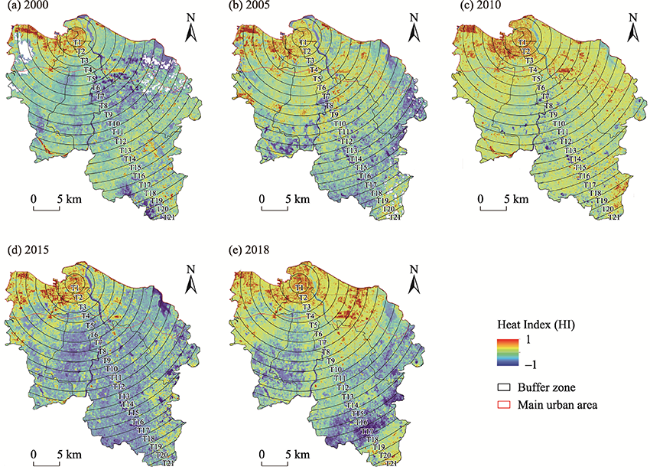
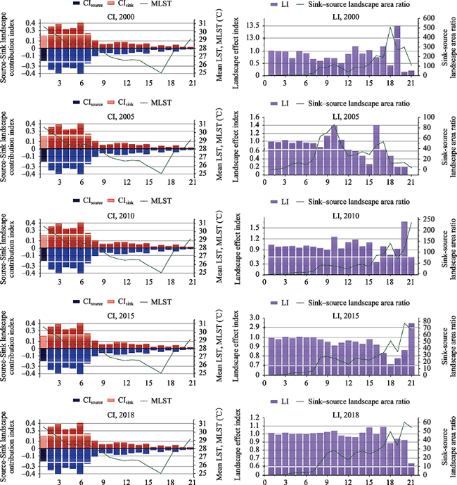
The Landsat images of the 2000, 2005, 2010, 2015, 2018 are selected as the data source to retrieve land cover and surface temperature data. The contribution of Sink-Source landscape pattern to the heat island and its ecological effects on urban and rural gradient were analyzed by using Heat Index (HI), Sink and Source Landscape Contribution (CIsink, CIsource) and Landscape Effect Index (LI) in Haikou. The results show that the heat island is concentrated on the West Coast, and in the central urban and Jiangdong New Area; the HI shows a pattern of decreasing value with the following land types: “Bare land>Artificial surface﹥Source landscape>Shrub grassland>Farmland>Sink landscape>Woodland>Water body”. In the central city section, the CIsink and CIsource are relatively large in these five periods. The LI decreases rapidly along the urban-rural gradient, promoting the Urban Heat Island (UHI) to a large degree. In contrast, the suburban area contributes to a lesser degree. Overall, the LI fluctuates, the proportion of mitigating UHI is large, and there is a second peak outside the city center. The existing Source-Sink Landscape contributes the most to UHI in the central urban area, and this contribution decreases along the urban-rural gradient. With the continuous expansion of city-town areas, the proportion of Sink areas has increased along the gradient, and the proportion of Source areas has subsequently declined, resulting in the spatial transfer and diffusion of UHI. Therefore, a UHI mitigation strategy based on the theory of regional landscape systems is proposed here.
LI Yujie , FU Hui . The Heat Island Effect Response to the Urban Landscape Pattern of Haikou based on the “Source-Sink” Theory[J]. Journal of Resources and Ecology, 2022 , 13(2) : 257 -269 . DOI: 10.5814/j.issn.1674-764x.2022.02.009
Table 1 POI data classification statistics |
| Year | Line code | Sensor | Date | Land cloud cover (%) |
|---|---|---|---|---|
| 2000 | 12446 | Landsat_5TM | 2000-06-19 | 13.00 |
| 2005 | 12446 | Landsat_5TM | 2005-06-17 | 11.00 |
| 2010 | 12446 | Landsat_5TM | 2010-07-27 | 8.00 |
| 2015 | 12446 | Landsat_8OLI_TIRS | 2015-06-26 | 0.78 |
| 2018 | 12446 | Landsat_8OLI_TIRS | 2018-06-21 | 0.48 |
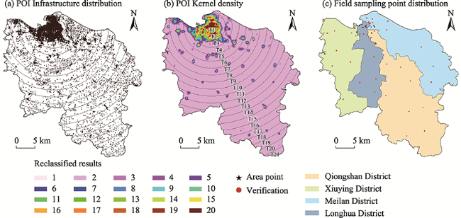
Fig. 3 Distribution and density of POI and distribution of field sampling points in research areaNote: The numbers in the legend represent the reclassification results based on kernel density analysis and larger numbers indicate higher kernel density. |
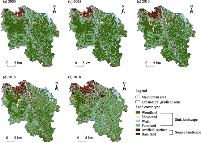
Fig. 1 Distribution of source and sink landscapes along the urban-rural gradient in 2000, 2005, 2010, 2015 and 2018.Note: T1-T21 mean the 21 gradient zones. |
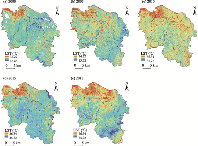
Fig. 2 LST for 2000, 2005, 2010, 2015 and 2018 in the study area. |
Table 2 POI data classification statistics |
| Service radius (m) | POI category | Number of effective points | Kernel density search radius (m) |
|---|---|---|---|
| 300-500 | Catering, Resident services, Education and culture | 20074 | 400 |
| 500-1000 | Wholesale and retail, Financial insurance, Automobile sales and services | 23485 | 750 |
| 1000-1500 | Transportation and storage, Public facilities, Commercial facilities and services, Sports and leisure, Accommodation, General hospitals | 14884 | 1250 |
| 1500-2000 | Health and social security, Agriculture, Forestry, Animal husbandry and fishery, Science and technology services, Scenic spots and golf, Park and squares | 1672 | 1750 |
| 2000-3000 | Villages, Towns, Areas of interest (university towns and international business districts) | 2551 | 2500 |
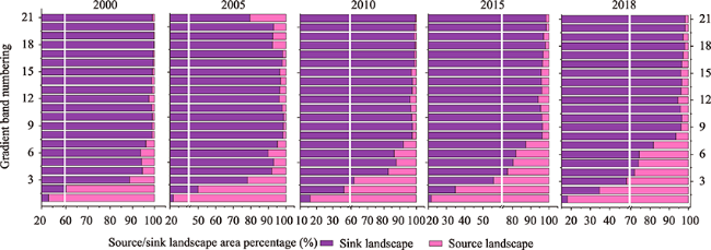
Fig. 4 Percentage landscape area change of sources and sinks |
Fig. 5 Distribution of HI along urban-rural gradients in 2000, 2005, 2010, 2015 and 2018. |
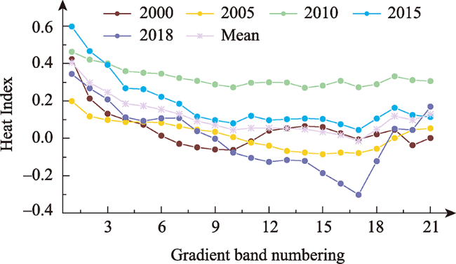
Fig. 6 Changes in MHI along the urban-rural gradient |
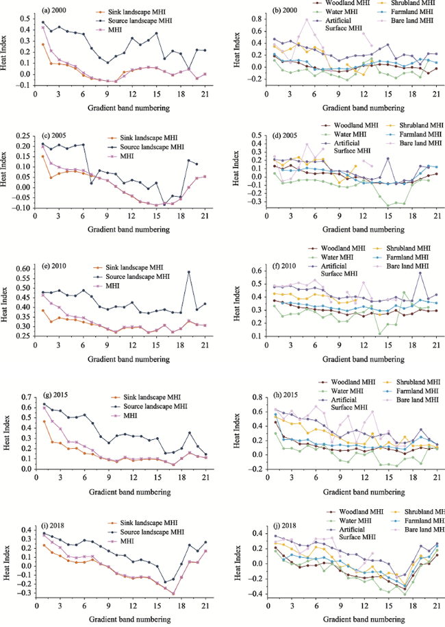
Table 3 HI characteristics of different Source-Sink landscape types |
| Year | Study area | Sink landscape | Woodland | Shrubland | Water | Farmland | Source landscape | Artificial surface | Bare land |
|---|---|---|---|---|---|---|---|---|---|
| 2000 | 0.0264 | 0.0092 | -0.0076 | 0.2938 | -0.0819 | 0.0355 | 0.3763 | 0.3687 | 0.4562 |
| 2005 | 0.0158 | 0.0049 | -0.0013 | 0.1817 | -0.0928 | 0.0226 | 0.1749 | 0.1733 | 0.1929 |
| 2010 | 0.3160 | 0.3008 | 0.2854 | 0.4022 | 0.2532 | 0.3219 | 0.4632 | 0.459 | 0.4905 |
| 2015 | 0.1635 | 0.1198 | 0.0839 | 0.3515 | 0.0112 | 0.1402 | 0.4931 | 0.4846 | 0.5613 |
| 2018 | -0.0104 | -0.0532 | -0.0963 | 0.1538 | -0.0983 | -0.0438 | 0.2542 | 0.2544 | 0.2525 |
Fig. 7 Changes of mean HI of urban and rural gradients in different source and sink landscapes in 2000-2018 |
Fig. 8 Source and sink landscapes contribution index (CI) and landscape effect index (LI)Note: The x-axis of all analysis graphs indicates the gradient band number. |
Table 4 Correlation between LI and Sink-Source landscape area ratio |
| Year | 2000 | 2005 | 2010 | 2015 | 2018 | 2000-2018 |
|---|---|---|---|---|---|---|
| Pearson correlation coefficient | 0.24 | 0.348 | -0.352 | 0.345 | -0.539* | 0.241* |
| Kendall correlation coefficient | -0.2 | 0.063 | -0.248 | -0.524** | -0.19 | -0.195** |
| Spearman correlation coefficient | -0.219 | 0.155 | -0.355 | -0.631** | -0.295 | -0.245* |
Note: ** and * indicate significant correlation at 0.01 and 0.05 levels (two-sided), respectively. |
Table 5 Correlation between MHI and Sink-Source landscape area ratio |
| Year | 2000 | 2005 | 2010 | 2015 | 2018 | 2000-2018 |
|---|---|---|---|---|---|---|
| Pearson correlation coefficient | -0.342 | -0.460* | -0.426 | -0.588** | -0.449* | -0.174 |
| Kendall correlation coefficient | -0.390* | -0.495** | -0.495** | -0.514** | -0.448** | -0.264** |
| Spearman correlation coefficient | -0.517* | -0.655** | -0.626** | -0.631** | -0.544* | -0.377** |
Note: ** and * indicate significant correlation at 0.01 and 0.05 levels (two-sided), respectively. |
We would like to thank Elizabeth Tokarz at Yale University for her assistance with English language and grammatical editing.
| [1] |
|
| [2] |
|
| [3] |
|
| [4] |
|
| [5] |
|
| [6] |
|
| [7] |
|
| [8] |
|
| [9] |
|
| [10] |
|
| [11] |
|
| [12] |
|
| [13] |
|
| [14] |
|
| [15] |
|
| [16] |
|
| [17] |
|
| [18] |
|
| [19] |
|
| [20] |
|
| [21] |
|
| [22] |
|
| [23] |
|
| [24] |
|
| [25] |
|
| [26] |
|
| [27] |
|
| [28] |
|
| [29] |
|
| [30] |
|
/
| 〈 |
|
〉 |