Ecosystem and Climate Change

Spatio-temporal Rainfall Distribution and Markov Chain Analogue Year Stochastic Daily Rainfall Model in Ethiopia

  • Nurilign SHIBABAW ,
  • Tesfahun BERHANE , * ,
  • Tesfaye KEBEDE ,
  • Assaye WALELIGN
Expand
  • Department of mathematics, Bahir Dar University, Bahir Dar, P.O. Box 79, Ethiopia
* Tesfahun BERHANE, E-mail:

Nurilign SHIBABAW, E-mail:

Received date: 2021-02-10

  Accepted date: 2021-06-18

  Online published: 2022-03-09

Abstract

This paper aims at the spatiotemporal distribution of rainfall in Ethiopia and developing stochastic daily rainfall model. Particularly, in this study, we used a Markov Chain Analogue Year (MCAY) model that is, Markov Chain with Analogue year (AY) component is used to model the occurrence process of daily rainfall and the intensity or amount of rainfall on wet days is described using Weibull, Log normal, mixed exponential and Gamma distributions. The MCAY model best describes the occurrence process of daily rainfall, this is due to the AY component included in the MC to model the frequency of daily rainfall. Then, by combining the occurrence process model and amount process model, we developed Markov Chain Analogue Year Weibull model (MCAYWBM), Markov Chain Analogue Year Log normal model (MCAYLNM), Markov Chain Analogue Year mixed exponential model (MCAYMEM) and Markov Chain Analogue Year gamma model (MCAYGM). The performance of the models is assessed by taking daily rainfall data from 21 weather stations (ranging from 1 January 1984-31 December 2018). The data is obtained from Ethiopia National Meteorology Agency (ENMA). The result shows that MCAYWBM, MCAYMEM and MCAYGM performs very well in the simulation of daily rainfall process in Ethiopia and their performances are nearly the same with a slight difference between them compared to MCAYLNM. The mean absolute percentage error (MAPE) in the four models: MCAYGM, MCAYWBM, MAYMEM and MCAYLNM are 2.16%, 2.27%, 2.25% and 11.41% respectively. Hence, MCAYGM, MCAYWBM, MAYMEM models have shown an excellent performance compared to MCAYLNM. In general, the light tailed distributions: Weibull, gamma and mixed exponential distributions are appropriate probability distributions to model the intensity of daily rainfall in Ethiopia especially, when these distributions are combined with MCAYM.

Cite this article

Nurilign SHIBABAW , Tesfahun BERHANE , Tesfaye KEBEDE , Assaye WALELIGN . Spatio-temporal Rainfall Distribution and Markov Chain Analogue Year Stochastic Daily Rainfall Model in Ethiopia[J]. Journal of Resources and Ecology, 2022 , 13(2) : 210 -219 . DOI: 10.5814/j.issn.1674-764x.2022.02.004

1 Introduction

Rainfall is the main source of water for crop production and animal rearing in most parts of the world, especially in developing countries like Ethiopia (Mearns and Norton, 2009). Rainfall in Ethiopia is the result of multi-weather systems that include Subtropical Jet (STJ), Intertropical Convergence Zone (ITCZ), Red Sea Convergence Zone (RSCZ), Tropical Easterly Jet (TEJ) and Somali Jet (NMA, 1996). Location, intensity and direction of these weather systems lead to the variability of the amount and distribution of rainfall in the country (Berhanu et al., 2014). Rainfall is one of the most important random processes that affect human lives significantly. Therefore, stochastic rainfall model is important for observing the climate change studies, planning and management of water resources (Papalexiou and Koutsoyiannis, 2016). Because of the stochastic nature of rainfall, stochastic models are mainly used to describe the rainfall process. When the available observed rainfall data are inadequate, it is possible to use stochastic rainfall models to produce synthetic rainfall series which resembles the statistical properties comparable to those of existing records.
Agriculture is the back bone of Ethiopian economy, which contributes around 52% of the gross domestic product (GDP), source of 85% of foreign exchange earnings and job opportunists for about 80% of the population in the country (Gezie, 2019). Ethiopian agriculture is highly dependent on rainfall, with irrigation agriculture contribution is not more than 1% of the country’s total cultivated land. Hence, the amount and timely distribution of rainfall during the growing period are very important or crucial to agricultural production (Di Falco et al., 2012). Delay onset dates, occurrence in scarce amount and variability of rainfall has great contribution to the reduction of crop yield with a significant amount (Makombe et al., 2007). Rainfall variability usually results in a reduction of 20% production and 25% rise in poverty rates in Ethiopia (Hagosa et al., 2011). This rainfall variability has a great impact on the income of every households whose life is dependent on agriculture. In general, agriculture takes the first rank in the Ethiopian economy and it is extremely dependent on natural rainfall (Bewket, 2009). Therefore developing a stochastic rainfall model is very important for the country. As to the knowledge of the author, there is no such models that describe daily rainfall in Ethiopia.
Rainfall is a stochastic process with two components: a discrete part describing the probability of dry and wet days (occurrence and nonoccurrence of rainfall) and a continuous part describing the amount or the intensity of wet day’s rainfall. The probability dry, in general, can be easily assessed from empirical data as the ratio of the number of dry days over the total number of days, while the continuous part is usually modeled by a parametric continuous distribution fitted to nonzero values (Papalexiou and Koutsoyiannis, 2016). However, this distribution is not unique. Different parametric distributions are used to model the amount of daily rainfall in literature, for instance the gamma, Weibull, exponential, generalized gamma, Burr Type XII, mixed exponential, kappa, Pearson Type-III (P3) and Log normal distributions are the most widely used distributions among others (Goncu, 2011; Papalexiou et al., 2012; Papalexiou and Koutsoyiannis, 2016).
In particular, gamma distribution has been used to model the intensity of daily rainfall in combination with mixed order Markov Chain (MC) (Stowasser, 2011). Exponential, gamma, Weibull, mixed exponential, generalized, Pareto distributions were used to simulate daily rainfall on wet days together with a lower order Markov Chain to describe the occurrence process of wet and dry days (Richardson, 1981). A first order Markov Chain in combination with a skewed normal distribution was used in order to model daily rainfall in north western part of Bangladesh (Rahman, 2000). First order Markov Chain and mixed exponential distribution to Model daily rainfall were considered by different scholars of them (Woolhiser and Pegram, 1979; Kannan and Farook, 2015). Pareto, Log normal, Weibull and gamma were proposed to model the amount of rainfall on wet days (Papalexiou et al., 2013).
The main objective of this study is to assess the spatiotemporal distribution of rainfall in Ethiopia and developing a stochastic daily rainfall model that appropriately describe dynamic nature of rainfall in Ethiopia. In this study, uniquely, we used Markov Chain Analogue Year (MCAY) that is a Markov Chain with Analogue Year component to model the occurrence process of daily rainfall in combination with four different probability distributions: gamma, Weibull, Log normal and mixed exponential distributions to model the amount of rainfall on wet days. The performance of these distributions is investigated especially when they are combined with MCAY model. The paper is structured as follows: In section 2 we have discussed materials and methods, section 3 presented spatiotemporal distribution of rainfall in Ethiopia, section 4 model formulation, in section 5 the obtained results are discussed under result and discussion and finally in section 6 we have made some concluding remarks.

2 Materials and method

Ethiopia is located in the Horn of Africa and covers an area of approximately 1.13×10⁶ km2. The topography of Ethiopia is highly diverse, with elevation ranging from 125 m below sea level at the Denakil Depression to 4620 m above sea level at Ras Dejen (Berhanu et al., 2014). More than 45% of the country is dominated by a high plateau East African Rift Valley. Regions with elevation greater than 1500 m is known as the highlands where almost 90% of the nation population is resides, perhaps to take advantage of its relatively disease-free environment (Devereux, 2001). Regions surrounding the highlands are known as lowlands (less than 1500 m), where most of the remaining population (mostly pastoralists) lives (Devereux, 2001). In this study, daily rainfall data from 21 weather stations with different altitudes ranging from 500 m to 3084 m above sea level are used to conduct this study. The weather stations are chosen based on the availability of fully recorded data from different parts of Ethiopia which includes North, South, East, West and Central part of the country). The daily rainfall data were collected from Ethiopia National Meteorology Agency (ENMA).
In this paper, the occurrence process of daily rainfall Xt and amount of daily rainfall Yt are modeled separately. Markov chain analogue year model (MCAYM) is used to model the occurrence process of daily rainfall and four different probability distributions are used to model the amount of daily rainfall and investigate their performance in describing the daily rainfall of Ethiopia. The occurrence and the amount model are combined to obtain a model for daily rainfall Rt on day t which is given as the product of the occurrence process Xt and the amount process Yt as given in equation (1). Both components of the daily rainfall model are described in detail in section 4.
${R_t} = {X_t}{Y_t}$
where, Rt is daily rainfall on day t; Xt denotes the occurrence process of daily rainfall and Yt represent the amount of rainfall on wet days.

3 Distribution of rainfall in Ethiopia

3.1 Spatial distribution of rainfall in Ethiopia

Mainly, the regional topography and seasonal evolution of the large-scale circulation determined the geographical distribution of rainfall in Ethiopia (Diro et al., 2011). Global and regional change of the weather systems and the topographic variation together with the seasonal cycles are reason or major cause for the spatial variability of rainfall in Ethiopia (Berhanu et al., 2013). For instance, the intensity of the mean annual rainfall in the southeast, east, and northeast borders of the country is lower by as much as less than 200 mm. The central and western highlands of the country receive an annual mean rainfall of more than 1200 mm.
In the northwest Kirmet (June to September) rainfall is in excess of 1000 mm, while in the southeast it is less than 100 mm. The mean annual rainfall of Ethiopia ranges from 141 mm in the arid area of eastern and northeastern borders of the country to 2275 mm in the southwestern highlands (Berhanu et al., 2013). The complex topographical and geographical features of the country have a strong impact on these spatial variations of climate and different rainfall Regimes in Ethiopia (Zeleke et al., 2013).

3.2 Seasonal distribution of rainfall in Ethiopia

Most of the areas in Ethiopia receives one main wet season locally known as Kirmet (from mid-June to mid-September) up to 350 mm per month in the wettest regions, when the intertropical convergence zone (ITCZ) is at its northernmost position (McSweeney et al., 2012). Northeaster and central part of Ethiopia also have a secondary wet season and considerably lesser, rainfall from February to May (called the Belge). The southern regions of Ethiopia experience two distinct wet seasons, which occur as the ITCZ passes through this to its southern position (Berhanu et al., 2014). The Belge season (March to May) is the main rainfall season yielding 100 to 200 mm of rainfall per month, followed by a lesser rainfall season in October to December known as Bega (around 100 mm of rainfall per month (Berhanu et al., 2014). Most part of the eastern border of Ethiopia receives very little rainfall at any time of the year (McSweeney et al., 2012). These unimodal and bimodal rainfall systems are the base for classifying the country into three rainfall regimes commonly, these rainfall Regimes are named as Regime one, Regime two, and Regime three (NMA, 1996) (Fig. 1).
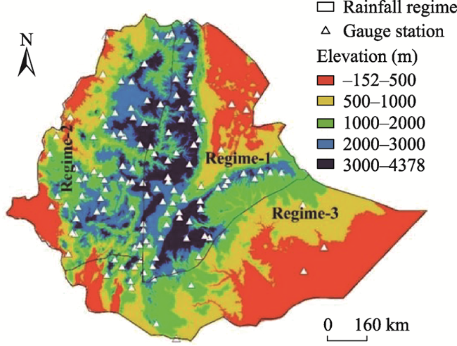
Fig. 1 Rainfall regimes in Ethiopia
Regime one comprises the central and the eastern part of the country and follows the bimodal rainfall system classi fied as the long rainy season or locally known as Kirmet (June-September) and short rains or locally known as Belge (March-May).
Regime two is a rainfall region in the western part of the country that covers from southwest to northwest and has a unimodal rainfall pattern (February-November). But the rainy period ranges are varied, if we go through southwest to northwest (see Fig. 2).
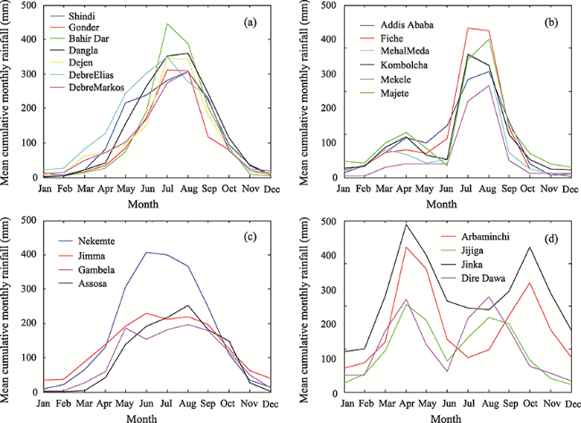
Fig. 2 Seasonal distribution of rainfall

Note: (a) Northwest part; (b) Central and Northeastern part; (c) Southwest section; (d) South and Southeast part of Ethiopia.

Regime three covers the south and southeastern parts of the country and has two distinct wet and dry seasons. In this rainfall regime, the main rainy season is from February- May and short rains from October to November and the dry periods are from June-September and December-February (Diro et al., 2009). Figure 2 illustrate the seasonal distribution of rainfall in different parts of Ethiopia which is presented by taking 21 weather stations from the three regimes.

4 Daily rainfall model

4.1 The occurrence process

Different researchers in literature used Markov chain to model the occurrence process of daily rainfall, to mention some (Caskey, 1963; Weiss, 1964; Kang et al., 2003; Kottegoda et al., 2004; Stowasser, 2011; Kannan and Farook, 2015). In this study, we use Markov chain with analogue year component (MCAY), to describe the occurrence process of daily rainfall. The reason behind using this the analogue year (AY) component is that the occurrence process of daily rainfall in the study area has significant positive correlation between two consecutive years. The correlation coefficient of the occurrence process of daily rainfall between consecutive years on average is 0.5551. As a result the MCAY model performs very well compared to the MC model.
The occurrence process Xt of a daily rainfall is modeled as:
${X_t} = \left\{ {\begin{array}{*{20}{c}}{0,}\\{1,}\end{array}\begin{array}{*{20}{c}}{\begin{array}{*{20}{c}}{}\end{array}{\rm{if}}\;{\rm{day}}\;t\;{\rm{is}}\;{\rm{dry,}}}\\{\;\begin{array}{*{20}{c}}{}\end{array}{\rm{if}}\;{\rm{day}}\;t\;{\rm{is}}\;{\rm{rainy}}{\rm{.}}}\end{array}} \right.$
Since daily rainfall occurrence varies with season, the transition probabilities are modelled to change daily within a year.
${\psi _{ti}} = {a_0} + \mathop \sum \limits_{k = 1}^{{m_i}} \left[ {{a_k}\cos \left( {\frac{{2\pi tk}}{{365}}} \right) + {b_k}\sin \left( {\frac{{2\pi tk}}{{365}}} \right)} \right];\;i = 1,2$
Where ${p^{01}} = {\psi _{t1}}$ (the transition probabilities from dry day to rainy day), ${\rm{\;}}{p^{11}} = {\psi _{t2}}$ (the transition probability from rainy day to rainy day), and mi determines the number of cosine and sine terms required to describe the seasonal cycles. To determine m we used the two common criteria for choosing model orders: the Akaike Information Criterion (AIC) (Akaike, 1974) and the Bayesian Information Criterion (BIC) (Schwarz, 1978). Here, based on the BIC, we choose m=2 for $p_t^{01}$ and m=4 for $p_t^{11}$; $p_t^{01}$ and $p_t^{11}$ represents the transition probability from dry day to wet day and from wet day to wet day respectively. Because the use of the BIC is generally preferable for sufficiently long time series data (over n=100) (Katz, 1981; Wilks, 2011).
The coefficients of the Fourier series are estimated by least squares method and the estimated coefficients are presented in Table 1 and 2. Due to the correlation exists between the same dates of two consecutive years, in this paper, in addition to the transition probability, we used the Analogue Year concept, that is, what was happened on the same date of the previous year. Which improves the accuracy of our models and it is given by equation (5). The occurrence process Xt can be generated recursively by comparing a uniform random variable ${u_{1,t}}\;~u\left( {0,1} \right)$ and the transition probabilities. Because the uniform random number U uniform on (0,1) is a random number between 0 and 1 analogous to the transition probabilities which have values between 0 and 1 and a starting value X0 (the first value of the observed data):
Table 1 Coefficients of ψt1
Coefficient ${a_0}$ ${a_1}$ ${a_2}$ ${b_1}$ ${b_2}$
Addis Ababa 2.837 -0.758 1.575 -3.094 0.252
Gonder 3.189 -1.888 1.569 -4.068 1.299
Jinka 3.667 -0.124 1.228 -0.803 1.451
Table 2 Coefficients of ψt2
Coefficient ${a_0}$ ${a_1}$ ${a_2}$ ${a_3}$ ${a_4}$ ${b_1}$ ${b_2}$ ${b_3}$ ${b_4}$
Addis Ababa 2.837 -0.756 1.575 -0.957 0.218 -3.094 0.252 0.419 -0.263
Gonder 3.189 -1.888 0.570 -0.958 0.499 -4.068 1.299 0.272 -0.324
Jinka 3.667 -1.228 0.631 -0.957 0.803 -1.451 0.184 0.116 -0.102
For $1 \le t \le 365$
${X_t} = \left\{ {\begin{array}{*{20}{c}}{1,\;{\rm{if}}\;p_t^{x1} \ge {u_{1,t}}}\\{0,\;{\rm{otherwise }}}\end{array}} \right.$
And for $366 \le t \le n$
${X_t} = \left\{ {\begin{array}{*{20}{c}}{1,\;{\rm{if}}\;{Z_t} \ge {r_{{\rm{min}}}}\;{\rm{and}}\;p_t^{x1} \ge {u_{1,t}}}\\{0,\;\;\;\;\;\;{\rm{otherwise}}\;\;\;\;\;\;\;\;\;\;\;\;\;\;\;\;\;\;}\end{array}} \right.$
where ${p^{x1}}$ is an abbreviation for $p_t^{01}$ and $p_t^{11},\;{Z_t} = X_{\left( {t - 365} \right)}^h$ and ${X^h}$ the historical (observed) rainfall on day t and $\;{r_{{\rm{min}}}}$ describes the minimal amount that is detected as rain. Table 1 and Table 2 reveal the parameters of the Fourier series in equation (3) for Addis Ababa, Gonder and Jinka rainfall respectively.

4.2 Amount process

To model the amount of daily rainfall we used four continuous probability distributions; gamma, Weibull, mixed and Log normal distributions. The gamma distribution function is a continuous probability distribution with shape parameter α and scale parameter β which is defined by the following probability density function (PDF)
$f\left( {x;\alpha,\beta } \right) = \frac{{{{\left( {\frac{x}{\beta }} \right)}^{\alpha - 1}}\exp ( - \frac{x}{\beta })}}{{\beta \Gamma {\rm{(}}\alpha {\rm{)}}}}$ for $x > 0,\alpha > 0,\beta > 0$
where α is the shape parameter, β is the scale parameter and $\Gamma ({\rm{\alpha }})$ is the gamma function given by
$\Gamma (\alpha ) = \mathop \smallint \limits_0^\infty {t^{\alpha - 1}}{{\rm{e}}^{ - t}}{\rm{d}}t$
The shape parameter α, determines the level of positive skewness and the scale parameter β, determines the spread of values, stretching when α is large and squeezing when β is small. Due to flexible representation of variety of distribution shapes which involves only two parameters, the gamma distribution commonly used to describe rainfall amount and assumed to be appropriate distribution to represent it (Stern and Coe, 1984; Wilks, 1990; Wilby et al., 1994; Rosenberg et al., 2004; Piantadosi et al., 2009). The appropriateness of the Gamma distribution to model rainfall amount has been proven by different scholars (Groisman, 1999; Katz, 1999; Guida et al., 2006; Ines and Hansen, 2006; Zolina, 2008; Block, 2009; Piani et al., 2010). The other distribution used in this study is the Weibull distribution which is considered as the generalization of exponential distribution is one of the common distributions in hydrology and its probability density is defined as:
$f\left( {x;{\lambda _1},{\lambda _2}} \right) = \frac{{{\lambda _1}}}{{{\lambda _2}}}{\left( {\frac{x}{{{\lambda _2}}}} \right)^{{\lambda _1} - 1}}\exp \left( { - \left( {\frac{x}{{{\lambda _2}}}} \right)} \right)$
and the cumulative distribution (CDF) is given by
$F\left( {x;{\lambda _1},{\lambda _2}} \right) = \exp \left( { - {{\left( {\frac{x}{{{\lambda _2}}}} \right)}^{{\lambda _1}}}} \right)$
Where ${\lambda _1}$ is the shape parameter and ${\lambda _2}$ is the scale parameter of the distribution. Weibull distribution used to model the intensity of daily rainfall by different scholars, for instance (Husak et al., 2007; Udomboso et al., 2010; Papalexiou et al., 2013).
Log normal distribution is one of the common distributions in hydrology and it is defined by the following probability density
${f_{LN}}\left( {x;{\beta _1},{\beta _2}} \right) = \frac{1}{{\sqrt \pi {\beta _1}x}}{\rm{exp}}\left( { - {{\ln }^2}{{\left( {\frac{x}{{{\beta _2}}}} \right)}^{\frac{1}{{{\beta _1}}}}}} \right)$
and the cumulative probability density is
${F_{LN}}\left( {x;{\beta _1},{\beta _2}} \right) = \frac{1}{2}{\rm{erf}}\left( {{{\ln }^2}{{\left( {\frac{x}{{{\beta _2}}}} \right)}^{\frac{1}{{{\beta _1}}}}}} \right)$
Where ${\beta _1}$ is the shape parameter, ${\beta _2}$is the scale parameter and $\;{\rm{erf}}\left( x \right) = \frac{2}{{\sqrt {\rm{\pi }} \mathop \smallint \nolimits_x^\infty {{\rm{e}}^{ - {t^2}}}{\rm{d}}t}}$. The distribution comprises the scale parameter ${\beta _2} > 0$ and the parameter ${\beta _1} > 0$ that controls the shape and the behavior of the tail. Lognormal is also considered a heavy-tailed distribution (it belongs to the sub-exponential family). The other most commonly used distribution in hydrology is the mixed exponential distribution (Woolhiser and Pegram, 1979; Woolhiser et al., 1982; Wilks and Wilby, 1999; Odening et al., 2007; Goncu, 2011; Kannan, and Farook, 2015; Berhane, 2020).
Mixed exponential distribution is a combination of two exponential distributions that inherits their properties and it has probability density (PDF)
${f_{mix}}\left( {x;\gamma,{\mu _1},{\mu _2}} \right) = \frac{\gamma }{{{\mu _1}}}\exp \left( { - \frac{x}{{{\mu _1}}}} \right) + \frac{{1 - \gamma }}{{{\mu _2}}}\exp \left( { - \frac{x}{{{\mu _2}}}} \right)$
with $0 \le {\mu _1} \le {\mu _2}$ and $0 \le \gamma \le 1$ and the cumulative density function (CDF) is defined by
${F_{mix}}\left( {x;\gamma,{\mu _1},{\mu _2}} \right) = \gamma \exp \left( { - \frac{x}{{{\mu _1}}}} \right) + \left( {1 - \gamma } \right)\exp \left( { - \frac{x}{{{\mu _2}}}} \right)$
where ${\mu _1}$ and ${\mu _2}$ are the parameters of the two exponential distribution respectively which represents the mean of the component distributions and $\gamma$ is the mixing parameter. Here, the maximum likelihood estimator (MLE) is used for parameter estimation because this approach performs much better than other methods (Wilks, 2011). To maintain the seasonal variation of daily rainfall amount, all the parameters of gamma and Weibull probability distributions are determined for each 12 calendar months individually in order that it varies monthly within a year and remains constant across different years, that is, for each month, we find its own distribution parameters.

5 Result and discussion

Figure 3 shows the average number of wet days in each 12 calendar months. As clearly observed from this figure, the Markov chain analogue year (MCAY) captures the occurrence process of daily rainfall very well. For the purpose of demonstration (demonstrate graphically) (to make concise), here we consider or take three stations: one from each of the three rainfall regimes, Addis Ababa from regime one, Gonder from regime two and Jinka from regime three. In Tables 3-5 we present average daily rainfall for the three weather stations: Addis Ababa, Gonder and Jinka respectively. For instance, the observed average daily rainfall in August for Addis Ababa weather station is 7.9279 mm, while the estimated average daily rainfall using MCAYWBM, MCAYGM, MCAYMEM and MCAYLNM models are 7.9711 mm, 8.0064 mm, 7.9961 mm and 9.0812 mm respectively. Figures 4-5 present the average daily rainfall and average cumulative monthly rainfall using the four models respectively, as one can observe from these figures, MCAYGM, MCAYWBM and MCAYMEM describe the average daily rainfall and average cumulative monthly rainfall very well compared to MCAYLNM.
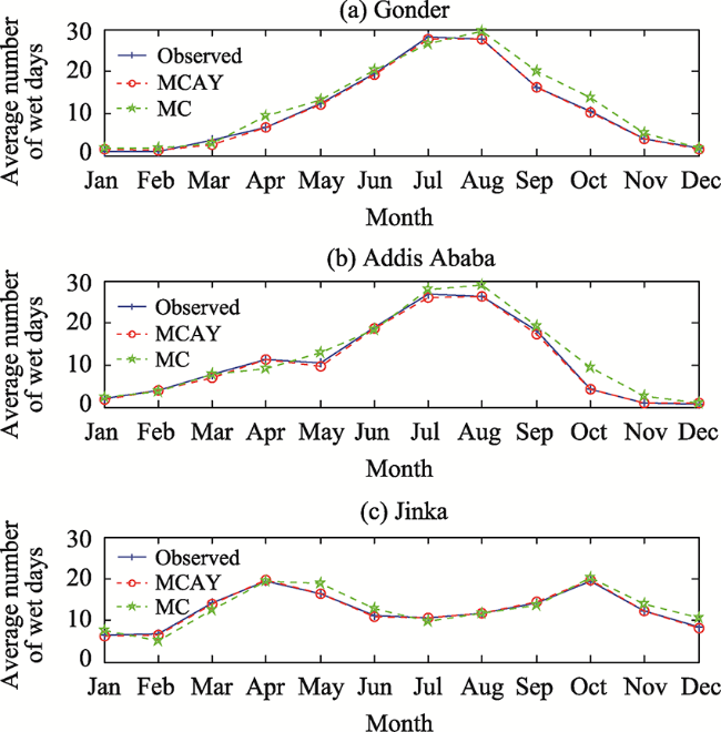
Fig. 3 Average number of wet days in each month for (a) Gonder, (b) Addis Ababa and (c) Jinka, Ethiopia.
The MCAYLNM shows a tendency of over estimation in the Kirmet season (June-September) in regime two and regime one that is northwest to southwest part and central section of Ethiopia and also March to July and October and November (mostly) in regime three (in south and southeast part of Ethiopia). In general Log normal shows a lesser performance in all stations (considered in this study) in the main rainy seasons in respective regimes compared to the other three models. The MAPE in MCAYGM, MCAYWBM, MCAYMEM and MCAYLNM are 2.16%, 2.27%, 2.25% and 11.41% respectively. In Table 6, we also presented the mean annual rainfall, for the three weather stations with the respective models, as clearly seen, MCAYLNM model perform less compared to the three models mentioned earlier. In this paper we use 10000 sample paths in the simulation process in order to reduce random sampling error.
Table 3 Average daily rainfall for Addis Ababa weather station in each of the four models and their corresponding absolute error (AE)
Models Observed value Simulated value
MCAYGM AE MCAYWBM AE MCAYMEM AE MCAYLNM AE
Jan 0.3609 0.3004 0.0605 0.2997 0.0612 0.3626 0.0017 0.3248 0.0361
Feb 0.9491 0.9895 0.0404 0.9911 0.0421 1.0108 0.0617 1.1309 0.1818
Mar 1.8816 1.7796 0.1020 1.7977 0.0839 1.7734 0.1082 1.9605 0.0789
Apr 3.0397 3.1513 0.1115 3.1702 0.1305 3.1410 0.1013 3.4277 0.3880
May 2.5981 2.5434 0.0547 2.5509 0.0472 2.4613 0.1368 2.6987 0.1006
Jun 4.0070 4.1037 0.0967 4.1209 0.1140 4.0833 0.0763 4.4320 0.4250
Jul 7.3475 7.4031 0.0556 7.3888 0.0413 7.3311 0.0236 8.3706 1.0231
Aug 7.9279 8.0064 0.0785 7.9711 0.0433 7.9961 0.0682 9.0812 1.1533
Sep 4.3583 4.2749 0.0835 4.2702 0.0881 4.2748 0.0836 4.7219 0.3635
Oct 1.0229 1.0009 0.0220 1.0104 0.0125 1.0180 0.0049 1.1613 0.1384
Nov 0.1404 0.1317 0.0087 0.1302 0.0102 0.1640 0.0236 0.1330 0.0074
Dec 0.2305 0.2595 0.0290 0.2642 0.0338 0.3150 0.0845 0.3072 0.0767
Table 4 Average daily rainfall for Gonder weather station in each of the four models and their corresponding absolute error (AE)
Month Observed value Simulated value
MCAYGM AE MCAYWBM AE MCAYMEM AE MCAYLNM AE
Jan 0.1145 0.1291 0.0147 0.1280 0.0135 0.1983 0.0839 0.1290 0.0145
Feb 0.1314 0.1928 0.0614 0.1933 0.0619 0.2208 0.0894 0.2090 0.0776
Mar 0.5148 0.4539 0.0609 0.4406 0.0742 0.4536 0.0612 0.4231 0.0917
Apr 1.0980 1.0106 0.0874 1.0029 0.0951 0.4536 0.0612 1.0652 0.0328
May 2.7638 2.7560 0.0079 2.7211 0.0427 2.7458 0.0181 2.8964 0.1326
Jun 5.8020 5.9059 0.1039 5.9128 0.1109 5.9047 0.1028 6.6651 0.8632
Jul 10.0538 10.2464 0.1925 10.2682 0.2144 10.2440 0.1902 11.6851 1.6312
Aug 9.9574 9.9019 0.0555 9.9273 0.0301 9.9106 0.0468 11.3244 1.3670
Sep 3.9097 3.9524 0.0428 3.9767 0.0670 3.9709 0.0613 4.4416 0.5319
Oct 2.5963 2.5378 0.0585 0.6640 0.0002 2.5196 0.0767 2.9164 0.3200
Nov 0.6643 0.6685 0.0042 2.5041 0.0922 0.6191 0.0452 0.7241 0.0598
Dec 0.3216 0.2899 0.0317 0.2865 0.0351 0.2847 0.0369 0.3007 0.0209
Table 5 Average daily rainfall for Jinka weather station in each of the four models and their corresponding absolute error (AE)
Month Observed value Simulated value
MCAYGM AE MCAYWBM AE MCAYMEM AE MCAYLNM AE
Jan 1.5350 1.4163 0.1187 1.4022 0.1328 1.4539 0.0811 1.5687 0.0337
Feb 1.8078 1.7229 0.0849 1.7280 0.0798 1.7364 0.0714 1.8371 0.0293
Mar 3.6064 3.6901 0.0838 3.6763 0.0700 3.6225 0.0162 3.9716 0.3653
Apr 6.5297 6.4680 0.0639 6.4538 0.0759 6.4622 0.0674 7.1270 0.5973
May 5.1542 5.2192 0.0650 5.2068 0.0527 5.2274 0.0732 5.8169 0.6627
Jun 3.5117 3.5050 0.0267 3.4826 0.0491 3.4727 0.0591 3.9712 0.4395
Jul 3.1684 3.3750 0.2066 3.3607 0.1923 3.2549 0.0864 3.7192 0.5508
Aug 3.1061 3.0507 0.0554 3.0345 0.0716 3.1035 0.0025 3.2733 0.1672
Sep 3.9003 3.9752 0.0749 3.9697 0.0694 4.0186 0.1183 4.4518 0.5515
Oct 5.4380 5.5533 0.1153 5.5095 0.0714 5.5651 0.1271 6.0701 0.6568
Nov 3.8471 3.9831 0.1360 3.9747 0.1276 3.9436 0.0966 4.5039 0.6568
Dec 2.2964 2.2254 0.0710 2.2134 0.0830 2.2365 0.0599 2.4757 0.1793
Table 6 Mean annual rainfall for Addis Ababa, Gonder and Jinka (mm)
Station Observed Simulated
MCAYGM MCAYWBM MCAYWBM MCAYLNM
Addis Ababa 1035.4 1038.3 1037.6 1038.4 1154.1
Gonder 1163.9 1167.3 1166.7 1166.3 1312.7
Jinka 1338.3 1346.5 1341.3 1343.9 1486.8
Figure 3 shows the average number of wet days for the three weather stations for Addis Ababa, Gonder and Jinka, Ethiopia. As one can observe from Fig. 3 and table 7, the Markov chain analogue year (MCAY) model has better performance compared to the Markov chain (MC) model in describing the occurrence process of daily rainfall.
Table 7 Mean absolute percentage error (MAPE) in describing the average number of wet days for Addis Ababa, Gonder and Jinka, Ethiopia (Unit: %)
Model Addis Ababa Gonder Jinka
MC 10.51 10.35 10.31
MCAY 2.22 2.33 1.99

6 Conclusions

In this study, we describe the spatiotemporal distribution of rainfall in Ethiopia and developed stochastic daily rainfall model. In particular, in this study we used Markov Chain Analogue year model (MCAY), that is, a Markov chain with Analogue Year component in combination with four different parametric distributions: Weibull, Log normal, mixed exponential and gamma distributions to model daily rainfall in Ethiopia. The combination of these two components (parts) of the daily rainfall models form MCAYWBM, MCAYLNM, MCAYMEM and MCAYGM. The MCAY model performs in an excellent way in describing the occurrence process of daily rainfall. This is mainly due to the Analogue Year component included in the Markov chain (MC) model. Further, the performance of the four distribu-tions, especially when combined with MCAY model has been investigated. The result shows that MCAYWBM, MCAYGM and MCAYMEM models have nearly the same performance in describing the daily rainfall with MAPE 2.27%, 2.16%, and 2.25% respectively while the Log normal distribution (or MCAYLN) model performs less compared to the other three models with MAPE 11.41%. In general, MCAYLN model performers less in all stations (used in this study) in relative to MCAYWBM, MCAYGM and MCAYMEM. Therefore, we can conclude that light tail distributions; Gamma, Weibull and mixed exponential distribution in combination with MCAY are more appropriate distributions to model the intensity of daily rainfall in Ethiopia compared to Log normal or heaver tail distributions.
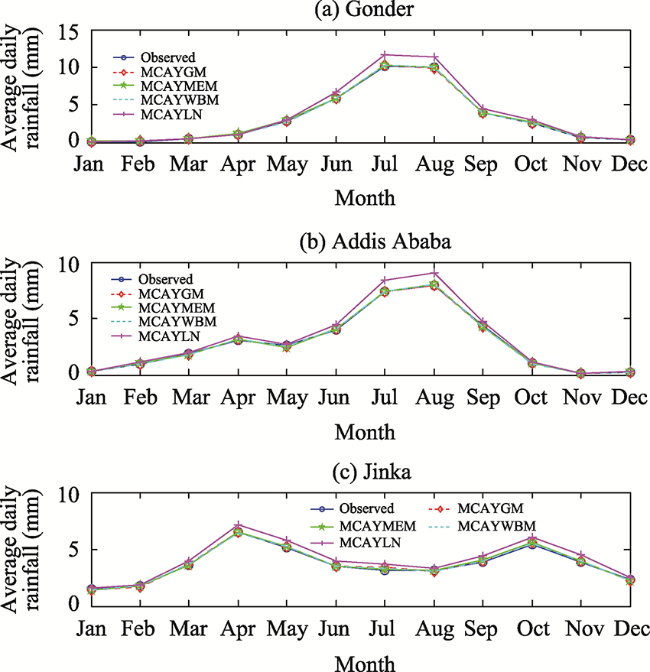
Fig. 4 Average daily rainfall for the 12 calendar months for (a) Gonder, (b) Addis Ababa and (c) Jinka, Ethiopia.
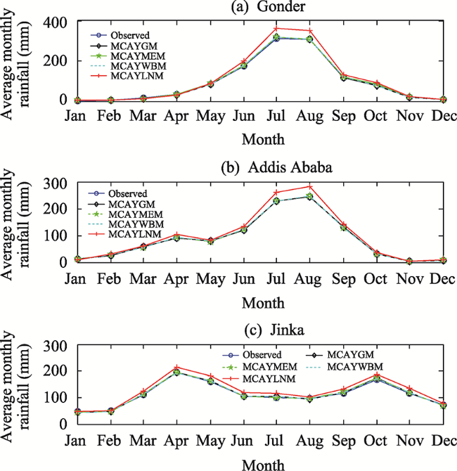
Fig. 5 Average cumulative monthly rainfall, for Gonder, Addis Ababa and Jinka, Ethiopia.
[1]
Akaike H. 1974. A new look at the statistical model identification. IEEE Transactions on Automatic Control, 19(6): 716-723.

DOI

[2]
Berhane T, Shibabaw N, Awgichew G, et al. 2020. Option pricing of weather derivatives based on a stochastic daily rainfall model with analogue year component. Heliyon, 6(1): e03212. DOI: 10.1016/j.heliyon.2020.e03212.

DOI

[3]
Berhanu B, Melesse A M, Seleshi Y. 2013. GIS-based hydrological zones and soil geo-database of Ethiopia. CATENA, 104: 21-31.

DOI

[4]
Berhanu B, Seleshi Y, Melesse A M. 2014. Surface water and groundwater resources of Ethiopia: Potentials and challenges of water resources development. In: Nile River Basin. Springer. DOI: 10.1007/978-3-319-02 720-3_6.

DOI

[5]
Bewket W. 2009. Rainfall variability and crop production in Ethiopia: Case study in the Amhara region. In: Proceedings of the 16th International Conference of Ethiopian Studies. Norwegian University of Science and Technology, Trondheim, Norway, 3: 823-836.

[6]
Block P J, Souza Filho F A, Sun L, et al. 2009. A streamflow forecasting framework using multiple climate and hydrological Models 1: JAWRA. Journal of the American Water Resources Association, 45(4): 828-843.

DOI

[7]
Caskey J E. 1963. A Markov chain model for the probability of precipitation occurrence in intervals of various length. Monthly Weather Review, 91(6): 298-301.

DOI

[8]
Devereux S. 2001. Livelihood insecurity and social protection: A re-emerging issue in rural development. Development Policy Review, 19(4): 507-519.

DOI

[9]
Di Falco S, Yesuf M, Kohlin G, et al. 2012. Estimating the impact of climate change on agriculture in low-income countries: Household level evidence from the Nile basin, Ethiopia. Environmental and Resource Economics, 52(4): 457-478.

DOI

[10]
Diro G T, Grimes D I F, Black E, et al. 2009. Evaluation of reanalysis rainfall estimates over Ethiopia. International Journal of Climatology, 29(1): 67-78.

DOI

[11]
Diro G T, Toniazzo T, Shaffrey L. 2011. Ethiopian rainfall in climate models. In: African climate and climate change, Dordrecht, Netherlands: Springer, 51-69.

[12]
Gezie M. 2019. Farmer’s response to climate change and variability in Ethiopia: A review. Cogent Food and Agriculture, 5(1): 1-13.

[13]
Goncu A. 2011. Modeling and pricing precipitation-based weather derivatives. Financial Mathematics and Applications, 1(1): 9-18.

[14]
Groisman P Y, Karl T R, Easterling D R, et al. 1999. Changes in the probability of heavy precipitation: Important indicators of climatic change. Climatic Change, 42(1): 243-283.

DOI

[15]
Guida D, Longobardi A, Villani P. 2006. Hydrological modelling for river basin management in a highly hydro-geological conditioned environment. WIT Transactions on Ecology and the Environment, 89. DOI: 10.2495/GEO060291.

DOI

[16]
Hagosa F, Makombe G, Namara R E, et al. 2011. Importance of irrigated agriculture to the Ethiopian economy: Capturing the direct net benefits of irrigation. Ethiopian Journal of Development Research, 32(1): 5-53.

[17]
Husak G J, Michaelsen J, Funk C. 2007. Use of the gamma distribution to represent monthly rainfall in Africa for drought monitoring applications. International Journal of Climatology, 27(7): 935-944.

DOI

[18]
Ines A V, Hansen J W. 2006. Bias correction of daily GCM rainfall for crop simulation studies. Agricultural and Forest Meteorology, 138(1-4): 44-53.

DOI

[19]
Kang S Z, Gu B J, Du T S, et al. 2003. Crop coefficient and ratio of transpiration to evapotranspiration of winter wheat and maize in a semi-humid region. Agricultural Water Management, 59(3): 239-254.

DOI

[20]
Kannan S K, Farook J A. 2015. Stochastic simulation of precipitation using Markov chain-mixed exponential model. Applied Mathematical Sciences, 65(9): 3205-3212.

[21]
Katz R W. 1981. On some criteria for estimating the order of a Markov chain. Technometrics, 23(3): 243-249.

DOI

[22]
Katz R W. 1999. Extreme value theory for precipitation: sensitivity analysis for climate change. Advances in Water Resources, 23(2): 133-139.

DOI

[23]
Kottegoda N, Natale L, Raiteri E. 2004. Some considerations of periodicity and persistence in daily rainfalls. Journal of hydrology, 296(1-4): 23-37.

DOI

[24]
Makombe G, Kelemework D, Aredo D. 2007. A comparative analysis of rain fed and irrigated agricultural production in Ethiopia. Irrigation and Drainage Systems, 21(1): 35-44.

DOI

[25]
McSweeney CMN LG. 2012. UNDP climate change country profiles Ethiopia. http://country-profiles.geog.ox.ac.ukAccessed 4 August 2013.

[26]
Mearns R, Norton A. 2009. The social dimensions of climate change:Equity and vulnerability in a warming world. Washington DC, USA: The World Bank.

[27]
NMA. 1996. Climatic and agro climatic resources of Ethiopia. National Meteorological Services Agency of Ethiopia. Meteorological Research Report Series, 1(1): 1-137.

[28]
Odening M, Musshoff O, Xu W. 2007. Analysis of rainfall derivatives using daily precipitation models: Opportunities and pitfalls. Agricultural Finance Review, 67(1): 135-156.

DOI

[29]
Papalexiou S, Koutsoyiannis D, Makropoulos C. 2012. How extreme is extreme? An assessment of daily rainfall distribution tails. Hydrology and Earth System Sciences Discussions, 9(5). DOI: 10.5194/hessd-9-5757-2012.

DOI

[30]
Papalexiou S M, Koutsoyiannis D, Makropoulos C. 2013. How extreme is extreme? An assessment of daily rainfall distribution tails. Hydrology and Earth System Sciences, 17(2): 851-862.

DOI

[31]
Papalexiou S M, Koutsoyiannis D. 2016. A global survey on the seasonal variation of the marginal distribution of daily precipitation. Advances in Water Resources, 94: 131-145.

DOI

[32]
Piani C, Haerter J O, Coppola E. 2010. Statistical bias correction for daily precipitation in regional climate models over Europe. Theoretical and Applied Climatology, 99(1-2): 187-192.

DOI

[33]
Piantadosi J, Boland J, Howlett P. 2009. Generating synthetic rainfall on various timescales daily, monthly and yearly. Environmental Modeling and Assessment, 14(4): 431-438.

DOI

[34]
Rahman M S. 2000. A rainfall simulation model for agricultural development in Bangladesh. Discrete Dynamics in Nature and Society, 5(1): 1-7.

DOI

[35]
Richardson C W. 1981. Stochastic simulation of daily precipitation, temperature, and solar radiation. Water Resources Research, 17(1): 182-190.

DOI

[36]
Rosenberg K, Boland J, Howlett P. 2004. Simulation of monthly rainfall totals. ANZIAM Journal, 46: 85-104.

DOI

[37]
Stern R D, Coe R. 1984. A model fitting analysis of daily rainfall data. Journal of the Royal Statistical Society: Series A (General), 147(1): 1-18.

[38]
Schwarz G. 1978. Estimating the dimension of a model. Annals of Statistics, 6(2): 461-464.

[39]
Stowasser M. 2011. Modelling rain risk: A multi-order Markov chain model approach. The Journal of Risk Finance, 13(1): 45-60.

DOI

[40]
Todorovic P, Woolhiser D A. 1975. A stochastic model of n-day precipitation. Journal of Applied Meteorology, 14(1): 17-24.

DOI

[41]
Udomboso C, Chubwu A, Nja M. 2010. The use of gamma and Weibull distributions in modeling rainfall data in Nigeria (a comparative analysis). Journal of Science Research, 9: 69-73.

[42]
Weiss L L. 1964. Sequences of wet or dry days described by a Markov chain probability model. Monthly Weather Review, 92(4): 169-176.

DOI

[43]
Wilby R, Greenfield B, Glenny C. 1994. A coupled synoptic-hydrological model for climate change impact assessment. Journal of Hydrology, 153(1-4): 265-290.

DOI

[44]
Wilks D S. 1990. Maximum likelihood estimation for the gamma distribution using data containing zeros. Journal of Climate, 3(12): 1495-1501.

DOI

[45]
Wilks D S. 2011. Statistical methods in the atmospheric sciences. San Diego, USA: Academic Press.

[46]
Wilks D S, Wilby R L. 1999. The weather generation game: A review of stochastic weather models. Progress in Physical Geography: Earth and Environment, 23(3): 329-357.

[47]
Woolhiser D A, Pegram G. 1979. Maximum likelihood estimation of Fourier coefficients to describe seasonal variations of parameters in stochastic daily precipitation models. Journal of Applied Meteorology, 18(1): 34-42.

DOI

[48]
Woolhiser D A, Roldan J. 1982. Stochastic daily precipitation models: 1. A comparison of occurrence processes. Water Resources Research, 18(5): 1451-1459.

DOI

[49]
Ye L, Hanson L S, Ding P Q, et al. 2018. The probability distribution of daily precipitation at the point and catchment scales in the United States. Hydrology and Earth System Sciences, 22(12): 6519-6531.

DOI

[50]
Zeleke T, Giorgi F, Tsidu G M, et al. 2013. Spatial and temporal variability of summer rainfall over Ethiopia from observations and a regional climate model experiment. Theoretical and Applied Climatology, 111(3-4): 665-681.

DOI

[51]
Zolina O, Simmer C, Kapala A, et al. 2008. Seasonally dependent changes of precipitation extremes over Germany since 1950 from a very dense observational network. Journal of Geophysical Research: Atmospheres, 113(6): 1-17.

Outlines

/