Ecosystems in Response to Global Change

Terrestrial Ecosystem Modeling with IBIS: Progress and Future Vision

  • LIU Jinxun , 1, * ,
  • LU Xuehe 2 ,
  • ZHU Qiuan 3 ,
  • YUAN Wenping 4 ,
  • YUAN Quanzhi 5 ,
  • ZHANG Zhen 6 ,
  • GUO Qingxi 7 ,
  • DEERING Carol 8
Expand
  • 1. U.S. Geological Survey, Western Geographic Science Center, Moffett Field, CA 94035, USA
  • 2. School of Geography Science and Geomatics Engineering, Suzhou University of Science and Technology, Suzhou, Jiangsu 215009, China
  • 3. College of Hydrology and Water Resources, Hohai University, Nanjing 210024, China
  • 4. School of Atmospheric Sciences, Sun Yat-sen University, Guangzhou 510275, China
  • 5. College of Geography and Resources Sciences, Sichuan Normal University, Chengdu 610068, China
  • 6. Department of Geographical Sciences, University of Maryland, College Park, MD 20742, USA
  • 7. School of Forestry, Northeast Forestry University, Harbin 150040, China
  • 8. KBR Inc., contractor to the U.S. Geological Survey, Earth Resources Observation and Science (EROS) Center, Sioux Falls, SD 57198, USA
* LIU Jinxun, E-mail:

Received date: 2021-08-16

  Accepted date: 2021-10-14

  Online published: 2022-01-08

Supported by

The Key Project of National Natural Science Foundation of China(41930651)

The National Natural Science Foundation of China(41871334)

Abstract

Dynamic Global Vegetation Models (DGVM) are powerful tools for studying complicated ecosystem processes and global changes. This review article synthesizes the developments and applications of the Integrated Biosphere Simulator (IBIS), a DGVM, over the past two decades. IBIS has been used to evaluate carbon, nitrogen, and water cycling in terrestrial ecosystems, vegetation changes, land-atmosphere interactions, land-aquatic system integration, and climate change impacts. Here we summarize model development work since IBIS v2.5, covering hydrology (evapotranspiration, groundwater, lateral routing), vegetation dynamics (plant functional type, land cover change), plant physiology (phenology, photosynthesis, carbon allocation, growth), biogeochemistry (soil carbon and nitrogen processes, greenhouse gas emissions), impacts of natural disturbances (drought, insect damage, fire) and human induced land use changes, and computational improvements. We also summarize IBIS model applications around the world in evaluating ecosystem productivity, carbon and water budgets, water use efficiency, natural disturbance effects, and impacts of climate change and land use change on the carbon cycle. Based on this review, visions of future cross-scale, cross-landscape and cross-system model development and applications are discussed.

Cite this article

LIU Jinxun , LU Xuehe , ZHU Qiuan , YUAN Wenping , YUAN Quanzhi , ZHANG Zhen , GUO Qingxi , DEERING Carol . Terrestrial Ecosystem Modeling with IBIS: Progress and Future Vision[J]. Journal of Resources and Ecology, 2022 , 13(1) : 2 -16 . DOI: 10.5814/j.issn.1674-764x.2022.01.001

1 Introduction

Terrestrial ecosystem carbon (C), nitrogen (N), and water (W) cycles are critical aspects of Earth’s biosphere function and represent fundamental ecosystem services to human beings. Over the past several decades, many empirical and process ecosystem models have been built to evaluate C, N, and W cycles from local to global scales. Complicated process-based models, including Dynamic Global Vegetation Models (DGVM) and Earth System Models (ESM), are currently the mainstream simulation tools for understanding and projecting possible future C, N, and W dynamics, and for tackling the complex issues of climate change and land use and land cover change (LUCC).
The Integrated Biosphere Simulator (IBIS) is a well- known, physically consistent DGVM. IBIS was originally developed by Foley et al. (1996). It has been further developed and used worldwide by many researchers and research groups. Since 1996, more than 350 peer-reviewed journal articles have been published describing applications of IBIS for various studies, including climate change, vegetation change, ecosystem productivity, C budget, water budget, and greenhouse gas (GHG) emissions. This paper provides an overview of the development and application of the IBIS model over the past two decades, covering additions of new biogeochemical processes to the model, pervasive model tests against observations, regional and global C and vegetation assessment, and technical computing improvements.

2 IBIS model framework and publication statistics

IBIS was developed as a first step toward gaining an im-proved understanding of global biospheric processes and studying their potential response to human activity (Foley et al., 1996). IBIS contains a wide range of biophysical and biogeochemical processes, including land surface physics, plant physiology and phenology, competition among vegetation types, and ecosystem C, N, and W cycling. IBIS not only simulates ecosystem mass and energy flows, but also includes many feedback controls among C, N, and W cycles.
The basic IBIS model frameworks were provided by Foley et al. (1996) and Kucharik et al. (2000). The major components and processes of the current IBIS (combination of multiple IBIS variants) are shown in Fig. 1, which is a slight modification of the Agro-IBIS model diagram (Kucharik, 2003).
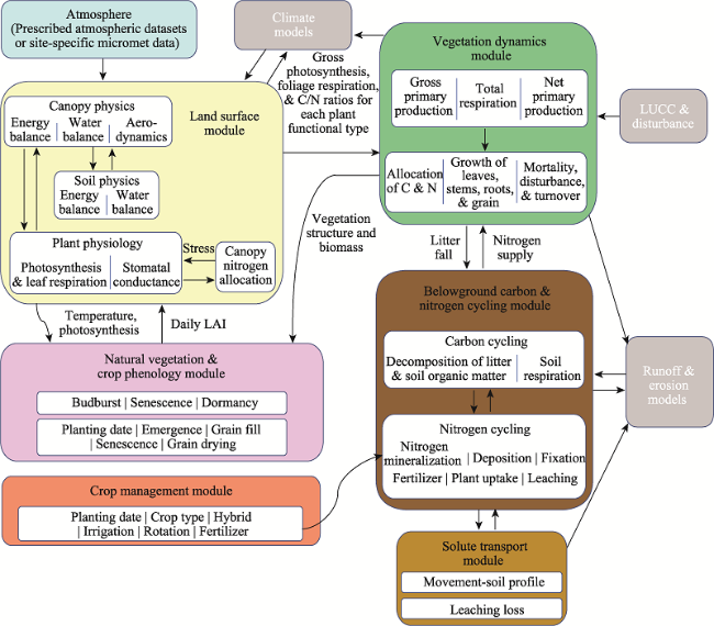
Fig. 1 IBIS key modules and their interactions (adopted and modified from Agro-IBIS)
Our search of the literature for IBIS related publications (in English or with English abstract), 1996 to 2021, returned approximately 600 journal article references. For our analysis, we extracted 357 records that directly applied either to the original IBIS model (IBIS v1.0 or IBIS v2.5) or a variant. Table 1 is a summary of these publications. In terms of geographic areas, North America (Canada-United States) tops the list of IBIS applied studies, followed up by global studies, and then by studies in China and the Amazon/Brazil. Both the original IBIS and several IBIS variants (as reflected in the model names) were used in these studies. Although many studies focused on forest and agricultural lands, most dealt with multiple/combined ecosystems. The research focus areas are wide-ranging and complex and therefore difficult to classify.
Table 1 Summary of IBIS model publications by study region, model name, ecosystem type, and research focus.
Application region Number of publications Model name Number of publications Ecosystem Number of publications Research focus* Number of publications
Canada-United States 98 IBIS 177 Multiple 173 Model Dev. 52
Global 70 Agro-IBIS 52 Forest land 93 Hydrology 36
China 67 CCM3-IBIS 23 Cropland 68 Vegetation 25
Amazon/Brazil 59 GENESIS-IBIS 9 Grassland 8 NPP 25
Africa 22 RegCM3-IBIS 9 Wetland 4 LUCC/Disturb. 23
India 19 MRCB-IBIS 9 Savanna 2 Phenology 11
Australia 3 TRIPLEX-GHG 8 Desert 1 Eco. Service 9
Europe 3 Can-IBIS 5 Oil sand 1 Nitrogen loss 6
Other 16 Other - Other - CH4/N2O 5

Note: *Summary of research focus is incomplete and represents only relative weights. NPP: Ecosystem net primary productivity; LUCC: Land use and land cover change.

In studies of the United States ecosystems, Agro-IBIS has been applied more often than IBIS or RegCM3-IBIS. Study topics covered ecosystem productivity, C and W cycles, climate change, and LUCC impacts. Almost all studies in Canada applied the Can-IBIS model in research on forest ecosystems. These studies were mainly at site scale and small region scale, with focuses on disturbance effects and climate change impacts. Seventy global-scale IBIS applications covered all major aspects of climate change, C and W cycles, ecosystem productivity, and vegetation change. Studies of ecosystems in China typically applied the original IBIS to study the C cycle, vegetation change, and climate change impacts. Wetland methane (CH4) simulations using TRIPLEX-GHG appeared in recent years. IBIS applications for the Amazon/Brazil region were related primarily to forest ecosystems, with considerations of LUCC and climate change. IBIS, Agro-IBIS, CCM3-IBIS, and other IBIS hybrids were the favored models. IBIS applications in Africa focused mainly on ET, runoff, and irrigation at large scales in savanna and cropland ecosystems, while applications in India concentrated mostly on forest ecosystems, especially vegetation change and ecosystem service. Only a few studies applied IBIS in Australia or Europe.

3 Major model development following IBIS v2.5

Over the years, various expansions of and improvements to IBIS have been implemented. The original IBIS model v1.0 (Foley et al., 1996) provided a list of model equations, covering canopy physiology, carbon balance, vegetation phenology, and vegetation dynamics. The IBIS v2.5 includes a soil biogeochemical module for dynamic soil C pools and fluxes, which the IBIS v1.0 does not. The v2.5 code and test data (Foley et al., 2005) have been archived and are publicly available on the website of the Oak Ridge National Laboratory Distributed Active Archive Center (ORNL DACC) for Biogeochemical Dynamics (https://daac.ornl.gov/MODELS/guides/IBIS_Guide.html).
Although IBIS development has continued world-wide, IBIS is not a community model. There is no central maintenance of the model development tree. Model codes are developed and maintained by different research groups. Currently, IBIS v2.6 is available on the SAGE website (https://nelson.wisc.edu/sage/data-and-models/model-code.php). Other IBIS variants are either downloadable from a public repository (e.g., pIBIS on https://github.com/jxliu2018/pIBIS) or accessible by contacting model developers (e.g., Agro-IBIS). Below, we summarize the IBIS model development with regard to eight aspects.

3.1 Vegetation phenology

The determination of vegetation existence and vegetation phenology in the original IBIS is based on the coldest temperature (TCMIN), thresholds for accumulated growing degree days (GDD), and threshold for 10-day average temperature (AVT10). For example, the existence of the temperate broadleaf cold-deciduous trees needs -45℃<TCMIN< 0℃, and annual GDD>1200 (GDD cumulation starts when temperature> 5 ℃); leaf expansion starts when AVT10> 0 ℃ and GDD reaches 100; and leaf senescence starts when AVT10 < 0 ℃.
Fu et al. (2014) optimized the GDD phenology parameters (beginning of growing season) of IBIS based on MODIS products and inversion tools. Fu et al. (2016) also tried to put a more accurate date on the end of growing season based on a critical temperature threshold (TcritTm) instead of relying on IBIS default temperature threshold values. They derived the TcritTm values (coefficients) of ten vegetation types globally by using MODIS remote sensing data. This modification is applicable globally and able to capture the trend, interannual variability, and spatial heterogeneity of phenology.
Other researchers looked at leaf area index (LAI) and growing season. The simulated monthly/seasonal LAI of IBIS is close to a trapezoidal or square shape (i.e., abrupt change). To improve modeling of leaf expansion and leaf fall, Cao et al. (2015) modified the IBIS leaf phenology algorithm with a hybrid approach using a logistic equation and a mass-balance mechanistic equation, where early leaf expansion relies on logistic growth. Then, the daily leaf biomass is used along with the original IBIS algorithm. The leaf-shedding phase relies on AVT10. Overall, the LAI of the whole growing season follows a bell-shaped curve. Most of the parameters, however, are localized just for the study region.
For crop phenology modeling, Sacks and Kucharik (2011) used Agro-IBIS and slightly modified the GDD calculation for United States Corn Belt states, enabling the calculation of different accumulated GDDs between corn planting time, reproductive period, and maturity time using an adjusted daily temperature between 10-30 ℃. They also added a gradual decline in the greenness fraction of leaves after the crop reaches the grain-fill period, and a leaf drying process from mature to harvest. Crop phenology/growth stage is determined by seasonal GDD accumulation. Base temperature of GDD calculation for different crops was set for soybean (8 ℃), maize (10 ℃), and wheat (0 ℃).

3.2 Photosynthesis, carbon allocation and growth

For canopy physiological processes, IBIS uses the Farquhar model to calculate ecosystem gross primary productivity (GPP) and net primary productivity (NPP). It uses constant values for carboxylation capacity (Vcmax) at 15 ℃. Improvements in GPP and NPP calculations were mostly on the parameter side, in particular the Vcmax setting for different crop species or wetland grasses. Castanho et al. (2013) added the spatial heterogeneity of Vcmax and the woody biomass residence time in IBIS and tested the model on the Amazon forest. The two parameters were found to be the most important properties determining the modeled spatial variation of above-ground NPP and biomass, respectively.
To incorporate a changing CO2 fertilization effect, Liu et al. (2011a) introduced an exponential decay function to get an adjusted CO2 level for the Farquhar equation in IBIS, which reduced CO2 growth enhancement on NPP to a more realistic range (7% NPP increase from 1951 to 2000). Similarly, Twine et al. (2013) modified Agro-IBIS to improve plant response to atmospheric CO2 by replacing IBIS default Vcmax values with new lower values calibrated at a soybean flux tower CO2 experiment site. The lower values were provided to accommodate the high CO2 concentration level (550 ppm).
Liu et al. (2005) modified the IBIS biomass growth calculation by directly applying a soil N availability modifier (Kp, a quadratic equation to approximate the Michaelis-Menten kinetics based on soil N level) to represent N constraints on biomass conversion, an additional step after canopy NPP calculation. In the original version of IBIS, the plant growth respiration ratio is an empirical constant and does not consider N limitation effects. Combining the constant growth respiration ratio and Kp implies a dynamic growth respiration ratio, or “biomass construction efficiency” ratio that relates canopy NPP to the production of stabilized biomass. This complies with the “Cyanide resistant path” of plant physiology that serves as an energy overflow when C supply exceeds demands, which means excessive C products from photosynthesis (e.g., sugar, starch, non-structural carbohydrates) cannot be converted to structural carbohydrates unless enough N is available.
IBIS v2.5 uses constant ratios to allocate NPP to leaf, wood, and root. Xia et al. (2015) integrated a C allocation model (resource availability model) into IBIS with satellite-derived LAI, which allows the model to inversely predict the allocation parameters for five deciduous vegetation types. The results showed that the C allocation coefficients can be reliably constrained by the satellite LAI product, and the new parameters in turn substantially improved model performance for simulating LAI and aboveground biomass globally. The spatial pattern of allocation coefficients among plant parts is supported by numerous studies. Compared with the standard version of the IBIS that uses fixed allocation coefficients, the revised resource availability C allocation model tends to promote higher C allocation to roots. As for root growth, Lu et al. (2019a) also modified IBIS by introducing a three-dimensional dynamic root growth model, in which explicit root architecture (i.e., fine and coarse roots) and root distribution are driven by soil W and N availabilities.

3.3 C:N ratio and N feedback controls

The C:N ratios of biomass and soil organic matter (SOM) in IBIS v2.5 are fixed values. Therefore, the N cycle was simply attached to the C cycle without N feedbacks. The Agro-IBIS model imposed additional leaf-level constraints on Vcmax (N stress) along with complete N-cycling, including fertilization, deposition, fixation (soybeans), mineralization, plant uptake and mechanistic leaching loss, and nitrate export (Donner et al., 2002; Donner and Kucharik, 2003; Kucharik, 2003; Kucharik and Twine, 2007).
Liu et al. (2005) applied dynamic C:N ratios to all the biomass and SOM pools in IBIS based on C:N ranges adopted from the CENTURY model (Parton et al., 1987). The N modification makes the modelled ecosystem responsive to dynamic N availability, resulting in N being a controlling factor on the whole C cycle. With this modification, the simulation of carbon budgets in the boreal forests in Saskatchewan, Canada, was improved (Liu et al., 2005).
Based on the hypothesis of negative N saturation effects on C assimilation, C allocation, and SOC decomposition (Aber et al., 1989), further modifications related to N saturation damage were made to improve simulation of the C-N coupling effects globally. Specifically, Lu et al. (2016) modified IBIS soil N control parameters (Kp, KI, and KM) to reflect the negative effects of N saturation when soil mineral N exceeds the saturation point (2 g N m-2).

3.4 Soil hydrology

IBIS v2.5 uses a prescribed allocation of root water uptake. Zheng and Wang (2007) used an empirical approach to represent the impact of dynamic water uptake by plant roots in IBIS. El Maayar et al. (2009) also developed a new scheme in which a dynamic allocation of root water uptake was simulated to compensate for the stress effect exerted by dry soil layers due to increasing water uptake from wetter layers. The dynamics of evapotranspiration and soil moisture were simulated with detailed root water uptake and root profile information.
In a later study, Soylu et al. (2014) connected the Hydrus-1D model to Agro-IBIS to examine the sensitivity of land surface evapotranspiration to the depth of the groundwater table, water movement, and groundwater representation. To evaluate the feedbacks between ecosystems and belowground hydrological processes, Zipper et al. (2017) integrated the MODFLOW model and the Agro-IBIS model. The study concluded that subsurface connections should be considered when evaluating hydrological impacts of land use change over different ecosystems. Ma et al. (2021) modified the IBIS model by incorporating an unfrozen water scheme for desert steppe, steppe, meadow, and wet meadow in the permafrost regions. Simulations of soil temperature, moisture, and NPP were significantly improved.
Coe and Foley (2001) used IBIS to look at hydrology and climate interactions. They connected a hydrological routing algorithm (HYDRA) to IBIS to evaluate the responses of hydrological processes to climate variability over the Lake Chad Basin. This extension of IBIS was also applied to simulate the river discharge and a flooded area of the Amazon/Tocantins River Basin (Coe et al., 2002). Kim and Eltahir (2004) considered topography’s effect and added the groundwater table (GWT) as a lower boundary in IBIS. They hypothesized that variations in elevation force similar variations in soil moisture. Their study improved hydrology simulation for a savanna ecosystem in West Africa, where the relatively wet valleys favor trees and the relatively dry hills favor grasses. Similarly, Gao and Zhang (2009) modified solar radiation calculations in IBIS by including terrain slope and aspect, which improved ET simulation.
Zeng et al. (2021) developed a revised model (IBISi) by integrating terrain influences and water distribution processes. Solar radiation and precipitation intensity were adjusted by a hillshade value and a terrain correction factor, respectively. A re-infiltration process of surface runoff within a pixel was integrated into a water distribution sub-module. Soil hydraulic conductivity was dynamically updated based on the saturated hydraulic conductivity, soil texture, and volumetric soil water content, instead of remaining at a constant value. The inverse migration of soil water due to surface evaporation was also integrated to simulate its impacts on soil moisture.

3.5 Soil organic matter decomposition

SOM decomposition simulation in IBIS v2.5 relies mainly on soil temperature and moisture. Liu et al. (2005) applied complicated N controls on SOM decomposition processes in IBIS based on studies of soil “preferential substrate utilization effect” (Merckx et al., 1987), “priming effect” (Dalenberg and Jager, 1989), and “competition effect” (Schimel et al., 1989). The overall effect is a negative feedback between soil C and N. When soil mineral N is abundant, more soil C can be preserved; but, when mineral N is insufficient, soil microorganisms will release more mineral N for plant growth by increasing SOM decomposition. Wang et al. (2017) combined the Microbial-ENzyme-mediated Decomposition (MEND) model with TRIPLEX-GHG and used a Michaelis-Menten equation to describe the enzyme-catalyzed soil C decomposition process. Guo and Guo (2013a) also improved the IBIS soil respiration module by adding a terrain analysis module, a modified soil water redistribution module, and the calculation of solar radiation received at the ground surface.

3.6 Methane and nitrous oxide emissions

IBIS v2.5 does not include CH4 and nitrous oxide (N2O) related processes. Zhu et al. (2014) incorporated a set of wetland CH4 processes into IBIS. The methanogenesis module consists of three major processes: CH4 production, CH4 transportation (ebullition, diffusion, and plant mediated transport), and CH4 oxidation. CH4 emission rates are determined by CH4 production and consumption in each soil layer. CH4 is produced in each soil layer when soil conditions are favorable. Changes in CH4 at each time-step in each soil layer are determined by CH4 production, oxidation, and three transport pathways. For each soil layer, the CH4 flux is the difference between the production and consumption/emission. For the wetland, soil water table dynamics were simulated based on an approach developed by Granberg et al. (1999). The modified IBIS (also called TRIPLEX-GHG) has been validated, modified, and applied to simulate CH4 emissions from site to global scales (Zhu et al., 2014, 2015, 2016, 2017). IBIS (TRIPLEX-GHG) was also used to study N2O, a principal greenhouse gas that has a relative global warming potential 298 times greater than that of CO2. Zhang et al. (2017) modeled nitrification and denitrification processes (i.e., N2O production, consumption, and diffusion) and quantified nitrous oxide emissions from natural forests and grasslands.
Song et al. (2020) developed a new process based biophysical model to quantify CH4 emissions from natural wetlands, which they integrated into IBIS. The new model includes CH4 production, oxidation, and transport processes (diffusion, plant-mediated transport, and ebullition). The new model uses several critical microbial mechanisms to represent the interaction of anaerobic fermenters, homoacetogens, hydrogenotrophic, acetoclastic methanogens, and methanotrophs in CH4 production and oxidation. The model was applied to 24 different wetlands globally with calibrations and sensitivity analysis. Results indicated that 1) For most sites, the model was able to capture the magnitude and variation of observed CH4 emissions under varying environmental conditions; 2) The parameters that regulate dissolved organic C, acetate production, and acetoclastic methanogenesis had significant impacts on simulated CH4 emissions; 3) The representation of the processes of CH4 cycling showed that CH4 oxidation was about half or more of CH4 production, and plant mediated transport was the dominant pathway at most sites; 4) The seasonality of simulated CH4 emissions can be controlled by soil temperature, water table position, or their combinations.

3.7 Plant functional types (PFT) and vegetation types

IBIS v2.5 provides an initial framework of vegetation type modeling, in which 12 basic PFTs (8 forests, 2 shrubs, and 2 grasses) are configured globally. In the Agro-IBIS development, typical C3 and C4 crops (e.g., soybean, spring and winter wheat, and maize) across the central United States were added (Kucharik, 2003). Sacks and Kucharik (2011) made further complicated crop PFT configurations in Agro-IBIS, dividing crop phenology into four phases determined by seasonal GDD accumulation. Van Loocke et al. (2010, 2012) added Miscanthus and switchgrass PFT to Agro-IBIS. Liu et al. (2016) added a simple crop production process in IBIS that included only two generic crop PFTs (C3 and C4 crops) based on existing grass PFT but changed the crop leaf biomass into straw and grain portions at year- end and did not consider crop planting/harvesting dates.
For forest ecosystems, Guo et al. (2010) modified IBIS PFTs to represent 6 common tree species in northern China, parameterized with local observation data. For wetlands, Zhu et al. (2014) added a new PFT in IBIS (TRIPLEX- GHG), adopting most of the phenological and physiological parameters from the C3 grass PFT in the original IBIS model, but incorporating new inundation-stress effects on GPP following the assumption made by Wania et al. (2009).

3.8 LUCC, management, and disturbances

IBIS v2.5 does not include a module for modeling LUCC effects, although it has a very simple subroutine for fire effects. IBIS modifications related to LUCC are extensive and include cropland, grassland, forest land, wetland, and urban areas (Twine et al., 2004; Li et al., 2007; Schneider et al., 2012; Liu et al., 2014; Cunha et al., 2015; Zhang et al., 2015; Mykleby et al., 2016; Sun et al., 2017).
Liu et al. (2016, 2020) used a parallel IBIS version (pIBIS) to quantify LUCC impacts on the C cycle. Eleven types of land conversions/disturbances were included: 1) Fire; 2) Logging; 3) Deforestation to grass/shrub; 4) Deforestation to cropland; 5) Afforestation from grass/shrub; 6) Afforestation from agriculture; 7) Urbanization from forest; 8) Urbanization from grass/shrub; 9) Urbanization from cropland; 10) Agricultural expansion (grass/shrub to cropland); 11) Agricultural contraction (cropland to grass/shrub). In pIBIS, C processes are mainly data driven. Extensive high-resolution wildfire severity data and LUCC data are used. Carbon fate following LUCC is based on removal ratios. Disturbed ecosystems are usually reset to an initial stage, except for fire and forest thinning.
Another focus of IBIS model expansion has been the effect of management. For cropping systems, modelled processes include crop rotations (Kucharik and Twine, 2007; El Maayar and Sonnentag, 2009), fertilizer application (Kucharik and Brye, 2003), irrigation (Marcella and Eltahir, 2014), and planting and harvesting (Kucharik, 2003; Sacks and Kucharik, 2011; Pires et al., 2016). For forests, the harvesting of bamboo was modeled by Lu et al. (2014). Liu et al. (2016) modelled forest logging using remote sensing data and modelled forest thinning based on thinning ratios derived from inventory data.
For disturbances, Chang et al. (2014) modelled drought and waterlogging effects in Can-IBIS for aspen forest dieback in western Canada. They used temporally and spatially explicit soil water stress constraints on the dynamic allocation of NPP and woody biomass turnover. The stress constraints are determined from the fraction of total fine-root biomass in the root layers, and the relative available soil water for plants. However, multi-year cumulative drought effects are not included. Damage from insect outbreak was later added to Can-IBIS by Landry et al. (2016), and mountain pine beetle (MPB) outbreak regimes on lodgepole pine in western North America forest over the past 240 years were quantified. The impacts on forest merchantable biomass, ecosystem C, surface albedo, and the net radiative forcing were modelled.

4 Model applications

Foley et al. (1996) used the IBIS v1.0 to perform a global 50-year simulation at 2-degree spatial resolution and produced ecosystem LAI and vegetation cover maps of near-equilibrium stage. Later, applications of IBIS v2.5, and other IBIS variants have covered wide-ranging geographies, numerous ecosystem types, and multiple research focuses. Studies of geographic regions and ecosystem types have been addressed above. Here we cover a few of the relatively large-scale applications among those research focuses.

4.1 Ecosystem productivity and vegetation growth

Twine and Kucharik (2009) used Agro-IBIS to analyze NPP trends from 1950 to 2002 over both natural and managed ecosystems in the central and eastern United States and concluded that climate changes have increased crop productivity in most agroecosystems. Twine et al. (2013) parameterized Agro-IBIS with field observations to simulate the response of soybean and maize in the central United States to an increase in atmospheric CO2 from 375 ppm to 550 ppm. They concluded that modifications of the Vcmax and specific leaf area are needed to avoid over-estimation of soybean yields at high CO2 levels.
Wang (2009) initialized IBIS with local fine root litterfall and mortality data and simulated the spatial pattern and seasonal variation of forest NPP in northern China. Yuan et al. (2014a) used IBIS to evaluate the NPP of China from 1961 to 2005 under normal climate conditions and concluded that the model is capable of reflecting the overall pattern of the NPP of China and that NPP estimates fell in the ranges of field observations as well as other model and remote sensing results. Yuan et al. (2017) followed up by quantitatively evaluating the NPP vulnerability to climate change in recent decades (1961-2015) and the near future (2016-2050) for China. Xue et al. (2017) looked at productivity at the global scale, using IBIS to evaluate the modeled GPP and potential aboveground biomass (AGB) and highlight the necessity of improving the specific plant functional type and meteorological inputs.

4.2 Ecosystem carbon budget

Zhang et al. (2013a) calculated the global terrestrial C budget (NEP, 3.3 Pg C per year during 2003-2009) as affected by spatially varying seasonal atmospheric CO2 using SCIAMACHY CO2 column data. Zhang et al. (2013b) applied the IBIS model to study the future carbon-water coupling with consideration of spatially varying atmospheric CO2 concentrations in China.
Liu et al. (2014) used IBIS to evaluate the C effects of China’s Grain for Green Program (GGP, reforestation) and concluded that areas converted from croplands to forests under the GGP could sequester 524.36 Tg C by 2100. The sequestration capacity showed substantial spatial variations, but with a large sequestration potential in southern China. The economic benefits of C sequestration from the GGP were also estimated based on current C price, which ranges from US $8.84 to US$44.20 billion from 2000 through 2100, and may exceed the current total GGP investment (US$38.99 billion). As the GGP program continues and forests grow, the impact of this program will be even larger in the future, making a more considerable contribution to China’s C sink.
Yang et al. (2016) evaluated the effects of climate change and elevated CO2 concentration on the temporal and spatial variation of the terrestrial ecosystem C budget in China from 1960 to 2006. They estimated that average NPP was 2.46 Pg C per year and had been increasing, while net ecosystem productivity (NEP) was 0.11 Pg C per year and had also been increasing. NPP and NEP were more correlated to precipitation than to temperature.
Liu et al. (2020) performed a 1-km resolution pIBIS simulation for the conterminous United States (CONUS) and concluded that although ecosystem NPP increased by approximately 12.3 Tg C per year during 1971-2015, most of it was offset by increased C loss from harvest and natural disturbance and increased ecosystem respiration related to forest aging. As a result, the strength of the overall ecosystem C sink (NBP, 170 Tg C per year) did not increase over time. The modeled results indicate the CONUS C sink was about 30% smaller than in previous modeling studies but converged more closely with inventory data.

4.3 Ecosystem water use efficiency, GHG emission

IBIS was used to evaluate the water use efficiency (WUE) of terrestrial ecosystems in China as related to climate change and heterogeneous atmospheric CO2 (Zhang et al., 2012, 2013b). IBIS was also used to simulate the effects of N deposition on WUE. Lu et al. (2019b) estimated that N deposition led to a global increase of 0.005 g C kg-1 H2O in WUE on average over the first decade of the 21st century, with spatial variabilities across the globe. The effects of N deposition on GPP determined the changes in WUE. In southeastern China, high N deposition led to decreased ET and consequently made WUE increase more significantly than in other parts of the world. Moreover, in southeastern China, the high N deposition enhanced the WUE under elevated CO2.
Zhu et al. (2014, 2015) used TRIPLEX-GHG to estimate spatially explicit wetland CH4 emissions of China (10-km) and the globe (0.5 degree). Zhang et al. (2016) simulated CH4 emissions of China under IPCC SERS A2, B1 scenarios and estimated that in the 21st century, the CO2 equivalent of annual plant CH4 emissions will be 83.18 Tg under the A2 scenario, and 77.34 Tg under the B1 scenario, accounting for 1.39% and 1.29% of China’s annual CO2 emissions, respectively.

4.4 Drought, fire, and land cover change impacts

Yuan et al. (2014b) used IBIS to characterize the impacts of long-term drought on terrestrial C fluxes in northern China and estimated a reduction of 0.05 Pg C yr-1 of average GPP during 1999-2011, as compared with 1982-1998. Zhang et al. (2011) also concluded that a dry climate was one of the critical factors impacting WUE in the Yangtze River Basin. Powell et al. (2013) studied Amazon forests subjected to experimental drought, and Pereira et al. (2020) studied the impact of drought on the Brazilian Dry Forest.
Botta and Foley (2002) applied IBIS to test the effects of climate variability and ecological disturbance rates on ecosystem composition and functioning of the Amazonian region, concluding that significant changes in soil and vegetation C stocks would occur. For the CONUS, Liu et al. (2020) simulated the wildfire and LUCC impacts on ecosystem C budget using pIBIS and summarized that clear-cut removals averaged 32 Tg C per year whereas forest thinning removed approximately 86 Tg C per year. Combustion of soil and biomass C was 6 Tg C per year during 1984-2000 but increased to 12 Tg C per year in the 2000s, and reached 25 Tg C per year during 2001-2015 with large interannual variation.

4.5 Other applications

Higgins (2007) used IBIS to study biodiversity loss in the Amazon as affected by climate change and LUCC. Yuan et al. (2011) simulated the potential natural vegetation distribution of China using IBIS after adjusting model parameter/threshold values, which increased vegetation mapping accuracy, especially on temperate broadleaf forest, needle-leaf forest, and grasslands. Sharma et al. (2017) reported the results of inherent as well as climate change driven vulnerability assessments for Indian forests across four indicators: biological richness, disturbance index, canopy cover, and slope. Booth et al. (2016) used Agro-IBIS as a biophysical model to show a process of translating scenario narratives to biophysical inputs.
Offline IBIS output data have been used as inputs for other models. Wang et al. (2008) used IBIS PFT to constrain the spatio-temporal patterns of forest CO2 exchange based on global eddy covariance measurements. Lassalle et al. (2009) used IBIS NPP to estimate the distribution of European diadromous fishes. Caldararu et al. (2016) evaluated global phenology using IBIS PFT. Huang et al. (2017) used it for forest site index evaluation in California. Faria et al. (2017) evaluated current and future patterns of fire-induced forest degradation in Amazonia with IBIS PAR.

5 Calibration and evaluation approaches

Model calibration is the process of fine-tuning model parameters with observation data. Model evaluation, typically undertaken after model calibration, assesses how well the model performs when checked against independent field data. Calibration of process-based IBIS models was conducted mostly at local scales, mainly because large-scale observation data are rarely available. Only a few existing large-scale (e.g., national scale) datasets have been used in IBIS calibration.

5.1 Flux tower, long-term research station

Local-scale data, such as flux tower measurements and field experiments, have been employed repeatedly for IBIS calibration. Delire and Foley (1999) used five sets of biophysical and hydrological measurements from across the globe to test IBIS soil moisture, temperature, surface energy fluxes, and CO2 fluxes of major ecosystem types. They confirmed that IBIS can adequately reproduce soil moisture and surface fluxes with a small number of site-specific parameter adjustments. El Maayar et al. (2001) tested IBIS on selected deciduous and boreal conifer forest stands in Canada by introducing an organic soil layer and calibrated modeled latent and sensible heat fluxes and NEP. Later, El Maayar et al. (2008) incorporated new root water uptake (RWU) and root profile schemes in IBIS and improved simulations of ET.
Kucharik et al. (2006) performed multiyear evaluations of IBIS at three AmeriFlux forest sites, focusing on vegetation structure, phenology, soil temperature, and CO2 and H2O vapor exchange. Later, Kucharik and Twine (2007) validated IBIS for crop systems using data from flux towers. They investigated soil temperature, net radiation, sensible and latent heat fluxes, crop growth, C allocation, phenology, biomass pools, heterotrophic respiration, and NEP. Kucharik and Twine concluded that if the impacts of surface residue management were not taken into account, inconsistent estimates of large-scale C and W exchange with the atmosphere may occur.
Chen et al. (2011) calibrated IBIS soil moisture dynamics, including ET, drainage, and runoff against field observations in Australia. Several researchers in China (Guo et al., 2010; Liu et al., 2011b, 2011c; Guo and Guo, 2013a, 2013b; Guo et al., 2019) used field data from a temperate forest long-term ecological research station in northern China to parametrize IBIS for NPP and soil respiration calculations. Lu et al. (2014) used flux tower observations to calibrate the NPP of bamboo forests in China.
Cunha (2013) used data from a Brazilian semiarid natural vegetation experimental site to calibrate the IBIS model’s PAR, sensible and latent heat fluxes, ET, and LAI, and concluded that IBIS, with a calibrated set of vegetation parameters, produced a considerably different energy balance from the default parameters. Liu et al. (2014) evaluated IBIS GPP against 62 eddy covariance sites around the world and found that the IBIS model is sensitive to Vcmax and that a large uncertainty exists in model parameterization. Overall, default IBIS parameters did not fit well with specific site observations, but with locally adjusted parameters, IBIS usually showed satisfying model behaviors.

5.2 Remote sensing

MODIS derived GPP, NPP, NDVI, FAPAR, and albedo products have been used to constrain IBIS parameters and state variables and to evaluate modeled results at regional and global scales. Xu et al. (2014) used MODIS NDVI and EVI for retrieving the phenology of temperate forests in the Agro-IBIS model and found that Agro-IBIS has different sensitivities to leaf onset and offset in terms of C assimilation. Xia et al. (2015) used MODIS satellite LAI products to invert IBIS allocation parameters for five deciduous vegetation types and improved model performance for simulating LAI and aboveground biomass globally. Senna et al. (2005) compared MODIS monthly FAPAR products with field measurements and IBIS simulations at an Amazonian tropical rain forest. Some of the other studies that compared IBIS phenology and MODIS data include Kim (2005), Twine and Kucharik (2008), Stöckli et al. (2008), Fu et al. (2014), and Chen et al. (2015).
Beyond MODIS data, Twine and Kucharik (2008) used AVHRR data to evaluate Agro-IBIS LAI simulation and suggested that AVHRR data may be used to evaluate the timing of onset and offset of the growing season of broadleaf crops and grasses. Zhang et al. (2013a, 2014) incorporated into IBIS the CO2 column observations from the SCIAMACHY (onboard European Space Agency ENVISAT satellite) to evaluate the spatio-temporal impact of CO2 concentration on the global C budget and WUE. Lu et al. (2016) used SCIAMACHY spatially explicit N2O column data to evaluate the effects of N saturation on the global C budget. Rondinelli (2015) used the Agro-IBIS model and USDA soil moisture network observations to evaluate near- surface soil moisture data from the SMOS (Soil Moisture and Ocean Salinity) satellite. Liu et al. (2020) used Landsat based MTBS wildland fire data to simulate fire emissions in the United States.

5.3 Inventory and census

Calibrations with inventory and census data were mostly applied at large scales. Kucharik et al. (2000) assembled a wide range of continental and global-scale data, including measurements of river discharge, NPP, vegetation structure, root biomass, soil C, litter C, and soil CO2 flux. Using these field data, their evaluation showed that simulated patterns of runoff, NPP, biomass, leaf area index, soil C, and total soil CO2 flux agreed reasonably well with measurements that have been compiled from numerous ecosystems. These results also compared favorably to other global model results. Yuan et al. (2011) validated IBIS potential vegetation type against the actual vegetation map of China at a 0.5 degree resolution and confirmed that IBIS vegetation classification matches with the existing inventory-based vegetation map. Yang et al. (2016) validated IBIS against forestry inventory and flux observation data for China. Liu et al. (2016, 2020) used county level observation data instead of site level data to calibrate the pIBIS model for CONUS. Data across 3100 counties included live biomass and dead wood from inventory, and crop yield from census. Comparison with MODIS NPP products was also at the county level instead of site level.

6 Technical developments

Very few publications focus on the technical side of the model development. Those authors who write about model technical developments typically include only brief mentions, although the efforts behind the developments were huge.

6.1 High performance computing (HPC) and parallel programing

IBIS HPC development evolved with advances in computing technology. Initial HPC applications focused mainly on shell script to allocate serial code and data to a number of PCs on local networks, or to multiple compute nodes on a cluster computer, such as in the cases of Can-IBIS and TRIPLEX-GHG that can be used on dozens to hundreds of CPUs.
Dennis et al. (2017) implemented the message passing interface (MPI) for Agro-IBIS using the modern parallel computing protocol, which can easily handle 1000 processors, although using 200-500 processors seemed more efficient. This development brought a 100-fold increase in performance, enabling domain scientists to work with intensive and complex ensemble simulations.
Most recently, even larger-scale MPI type parallel computing was implemented on the pIBIS model (Liu et al., 2020) using parallel NetCDF for reading inputs and collective parallel I/O for writing outputs. This approach can use 100000 processors on super large (peta-scale) computers, making it possible to perform large-region high-resolution C simulations (i.e., 1 km for the CONUS).

6.2 IBIS on Microsoft Windows platform

Guo and Guo (2013a) recoded IBIS using Visual C# and C++, enabling the model to run on the Microsoft Windows platform (Any use of trade, firm, or product names is for descriptive purposes only and does not imply endorsement by the U.S. Government). They also used Visual FoxPro 9.0 to develop a database to manage model parameters and model simulation results in ASCII format. All the site information, climate records, vegetation inventories and measurements, and daily/monthly/yearly simulation results are visually managed. In addition, they made necessary modifications on radiation of mountain terrain, species level forest PFT, and phenology. The modified IBIS performed well at stand, watershed, and regional scales.

6.3 Fast spin-up

One of the technical aspects of computing efficiency is the model’s spin-up process to gain balanced initial soil C pools. Liu et al. (2020) adopted the fast soil spin-up method of Xia et al. (2012), which compared input and output fluxes of a soil C pool each year. In pIBIS, when input and output C fluxes become very close, the soil C pool is close to a theoretical balanced state. However, one key feature of the pIBIS soil spin-up is the inclusion of the observed soil C pool value. While still using universal soil C decomposition parameters, a set of internal scalars are employed in the first 20 simulation years that dynamically adjust the slow soil C pool size, and then the slow C is deducted from the total observed soil C pool to obtain the size of the initial passive soil C pool. This avoids the unrealistic total soil C pool size after traditional spin-up in IBIS.

6.4 Pre- and post-processing

Pre- and post-simulation programs are seldom described in IBIS literature, although most versions have their own relevant codes. Here we give just a brief look at the procedures of pIBIS (Liu et al., 2020). The overall workflow of the current pIBIS includes: 1) A pre-simulation program that divides a large study region into sub-regions and calculates expected compute nodes for each sub-region. For example, the conterminous United States can be separated into 13 large sub-regions at 1-km resolution; 2) For a single sub- region, a decomposition program converts and combines all NetCDF inputs of various spatial resolutions (e.g., 1-km, 4-km, and 0.5 degree) into a 1-km pNetCDF dataset for parallel reading from each compute node. This step includes complicated data decomposition and spatial sampling/interpolation; 3) IBIS_lib performs the actual simulation; 4) After merging results into the whole region, when needed, a calibration program compares IBIS outputs with field observations and generates a set of scalars to adjust pIBIS parameters for a new simulation; 5) The final step includes a set of programs to perform spatial-temporal statistics and analysis, such as calculating NPP temporal trends on each land pixel and calculating NPP response to precipitation during a given period. External toolkits like R, SciDB, and ParaView may be used for wider and deeper data analysis.
As noted earlier in this review, no community model development mechanism exists for IBIS. Moreover, many of the IBIS versions are not publicly available. Cooperation among individual IBIS modelers, including sharing of the code and technical documentation, is helpful for further improving IBIS.

7 Future visions

The IBIS model has been used globally for many kinds of ecosystem and environmental studies. Most of the model applications have focused on the terrestrial C and W cycles along with climate change impacts and LUCC and disturbance effects. IBIS coupling to GCM is one modeling aspect that we did not discuss much in the review. Despite the fact that IBIS has undergone significant model expansions and refinements in recent years, and that hundreds of studies have applied IBIS and its extensions, further research attention is warranted in the following areas.

7.1 Forest simulation

Most forest biometric data and associated management activities (e.g., growth rate, mortality rate, stem density, thinning, logging, woody crop harvesting) are age related. However, none of the current versions of IBIS includes forest age as a factor. Consequently, IBIS overestimates forest recovery in the early years after logging. Introducing a forest age variable and including tree diameter, height, and stem density would likely enhance model calibration and assist with precise forest management strategies. This is more necessary now that management scale datasets from new satellite observations, such as NASA’s Global Ecosystem Dynamics Investigation (GEDI), are becoming available.

7.2 Cross-scale high-resolution model applications

Modeling of natural vegetation distribution and vegetation change are basic IBIS capabilities. However, most vegetation change happens slowly and unevenly. Observed vegetation movements (tree line shifts) are usually at meters (vertical) and hundred meters (horizontal) per year (Huntley, 1991; Grace et al., 2002; Kennedy, 2007). Similarly, wetland area variation and sea level rise-induced land loss have been occurring at high-resolution scales, as are the ecosystem productivities of coastal mangroves and marshes. Coarse resolution IBIS simulations cannot effectively reflect such vegetation and land over changes. In addition, long- term vegetation succession combined with rapid LUCC is difficult to simulate. Most of the global land areas are human managed/disturbed. Human land management activities are usually captured at management scales (e.g., 30-250 m). Therefore, cross-scale simulation is needed, i.e., using high resolution data (30-250 m) to improve vegetation modeling across large regions.

7.3 Cross-landscape lateral carbon and hydrology simulations

Cross landscape model simulations are usually difficult for process models because the model needs to consider communication (data exchange) among adjacent land pixels. Soil C erosion and deposition is one example. Redistribution of soil eroded C on the landscape each year to update the temporal process on each land pixel puts a heavy load on current typical computing resources. At a small scale, IBIS has been incorporated into the PALMS model for one-dimensional fluxes of energy, water, C and N simulation, and linking PALMS runoff and sediment transport calculations (Bonilla et al., 2007). But overall, IBIS research at the cross-landscape level has been very limited.

7.4 Cross-system land-aquatic consortium applications

Cross system simulation is a needed extension of the IBIS model. Not only do we need process models to simulate multiple ecosystems, but we also need to consider the C, N, and W fluxes between the systems. A particular focus should be the “land-aquatic consortium” that depicts the C transfer from the land system to the aquatic system. Li et al. (2019) used the TRIPLEX-HYDRA (a hybrid with IBIS) to model the global DOC flux in soil and DOC riverine transport, although spatial resolution is coarse (0.5 degree). For C cycle science, this is one of the most challenging areas.

7.5 Social-economic applications

IBIS can be used for C neutrality research to facilitate C projections under various climate and LUCC scenarios and help determine C credits and C trade.
(1) Ecosystem service: IBIS has been used in some ecosystem service evaluations in recent years (e.g., Lima et al., 2014; Ren et al., 2016; Strand et al., 2018; Qiu et al., 2020; Wang et al., 2020) because the model can produce output variables directly related to ecosystem services: among them food, timber, water quality, water resource conservation, ecosystem productivity, C sequestration, soil erosion/retention, GHG emission, biodiversity, and recreation. However, most applications are still at a coarse spatial resolution. High-resolution human-management-scale model evaluations are necessary because such ecosystem service simulations are likely to inform policy decisions regarding credits or awards (e.g., C credit to landowners).
(2) Climate change mitigation and adaptation policy: IBIS can be used for policy development. For example, Murthy et al. (2011) and Kumar et al. (2018) discussed forest type shifts in India (IBIS simulations) and related ecological and socioeconomic adaption policies. Donner and Kucharik (2008) used Agro-IBIS to show the conflicts of United States biofuel production policy and the N leaching from cropland to the Mississippi and Atchafalaya Rivers. GHG emission levels across the globe are also a concern. China has set a goal of achieving C neutrality by 2060. The target year for United States C neutrality is 2050. Policy makers are looking to science data and modeling to help shape, monitor, and evaluate GHG emissions targets such as these, and a recent study suggests that IBIS can be an important tool. Zhang et al. (2021) used IBIS to show that C sequestration of terrestrial ecosystems in China can offset about 10.0% to 82.5% of C emissions under the RCP60 scenario.

8 Conclusions

IBIS has been intensively calibrated at local scales and has proved to be an effective and versatile DGVM that can be applied from local to global scales. The model incorporates all the key processes within the terrestrial ecosystems and can be coupled with atmospheric chemistry/transport models and aquatic/erosion models. Since IBIS can be applied to various ecosystems with detailed vegetation processes, including land cover change and land management, it can be used to evaluate ecosystem C, N, and W cycles at human management scales and help land managers understand and manage ecosystem services. The IBIS modeling framework is also suitable for performing regional scale and global scale simulations, making it an ideal tool for performing national and global scale C assessments, climate impact evaluations, ecosystem vulnerability calculations, and other environmental analyses. Advances in parallel computing technology and existing and upcoming high-resolution remote sensing data hold much promise for future applications of IBIS. One drawback we see is that previous IBIS model developments have been individually implemented. There is no community model development mechanism to date. Integrating the many different IBIS variants into a new package will likely make the model even more powerful.

Work of Jinxun Liu and Carol Deering was funded by the U.S. Geological Survey Biologic Carbon Sequestration Assessment Program (LandCarbon).

[1]
Aber J D, Nadelhoffer K J, Steudler P, et al. 1989. Nitrogen saturation in northern forest ecosystems. BioScience, 39(6): 378-386.

DOI

[2]
Bonilla C A, Norman J A, Molling C C. 2007. Water erosion estimation in topographically complex landscapes: Model description and first verifications. Soil Science Society of America Journal, 71(5): 1524-1537.

DOI

[3]
Booth E G, Qiu J X, Carpenter S R, et al. 2016. From qualitative to quantitative environmental scenarios: Translating storylines into biophysical modeling inputs at the watershed scale. Environmental Modelling & Software, 85: 80-97.

[4]
Botta A, Foley J A. 2002. Effects of climate variability and disturbances on the Amazonian terrestrial ecosystems dynamics. Global Biogeochemical Cycles, 16(4): 18-1-18-11. DOI: 10.1029/2000GB001338.

DOI

[5]
Caldararu S, Purves D W, Smith M J. 2016. The effect of using the plant functional type paradigm on a data-constrained global phenology model. Biogeosciences, 13(4): 925-941.

DOI

[6]
Cao X, Zhou Z, Chen X, et al. 2015. Improving leaf area index simulation of IBIS model and its effect on water carbon and energy-A case study in Changbai Mountain broadleaved forest of China. Ecological Modelling, 303: 97-104.

DOI

[7]
Castanho A D A, Coe M T, Costa M H, et al. 2013. Improving simulated Amazon forest biomass and productivity by including spatial variation in biophysical parameters. Biogeosciences, 10(4): 2255-2272.

DOI

[8]
Chang K H, Price D T, Chen J M, et al. 2014. Simulating impacts of water stress on woody biomass in the southern boreal region of western Canada using a dynamic vegetation model. Agricultural and Forest Meteorology, 198-199: 142-154.

DOI

[9]
Chen M, Willgoose G R, Saco P M. 2011. Estimating temporal soil moisture dynamics using the HYDRUS-1D and IBIS models. In: Valentine E M (ed.). Balance and uncertainty-Water in a changing world. Proceedings of the 34th IAHR Congress. Brisbane, Australia: International Association of Hydraulic Engineering & Research, https://espace.library.uq.edu.au/view/UQ:243193.

[10]
Chen M, Willgoose G R, Saco P M. 2015. Investigating the impact of leaf area index temporal variability on soil moisture predictions using remote sensing vegetation data. Journal of Hydrology, 522: 274-284.

DOI

[11]
Coe M T, Costa M H, Botta A. 2002. Long-term simulations of discharge and floods in the Amazon Basin. Journal of Geophysical Research: Atmospheres, 107(D20): LBA 11-1-LBA 11-17. DOI: 10.1029/2001JD000740.

DOI

[12]
Coe M T, Foley J A. 2001. Human and natural impacts on the water resources of the Lake Chad Basin. Journal of Geophysical Research: Atmospheres, 106(D4): 3349-3356.

DOI

[13]
Cunha A P M A, Alvalá R C S, de Oliveira G S. 2013a. The impact of land cover change on land surface processes in the semiarid of Brazil. Revista Brasileira de Meteorologia, 28(2): 139-152.

DOI

[14]
Cunha A P M A, Alvalá R C S, Sampaio G, et al. 2013b. Calibration and validation of the integrated biosphere simulator (IBIS) for a Brazilian semiarid region. Journal of Applied Meteorology and Climatology, 52(12): 2753-2770.

DOI

[15]
Cunha A P M A, Alvalá R C S, Kubota P Y, et al. 2015. Impacts of land use and land cover changes on the climate over Northeast Brazil. Atmospheric Science Letters, 16(3): 219-227.

DOI

[16]
Dalenberg J W, Jager G. 1989. Priming effect of some organic additions to 14C-labelled soil. Soil Biology and Biochemistry, 21(3): 443-448.

DOI

[17]
Delire C, Foley J A. 1999. Evaluating the performance of a land surface/ ecosystem model with biophysical measurements from contrasting environments. Journal of Geophysical Research: Atmospheres, 104 (D14): 16895-16909.

DOI

[18]
Dennis H E B, Ward A S, Balson T, et al. 2017. High performance computing enabled simulation of the food-water-energy system. In: PEARC17. Proceedings of the practice and experience in advanced research computing 2017 on sustainability, success and impact. New Orleans, USA: The Association for Computing Machinery.

[19]
Donner S D, Coe M T, Lenters J D, et al. 2002. Modeling the impact of hydrological changes on nitrate transport in the Mississippi River Basin from 1955 to 1994. Global Biogeochemical Cycles, 16(3): 16-1-16-19. DOI: 10.1029/2001gb001396.

DOI

[20]
Donner S D, Kucharik C J. 2003. Evaluating the impacts of land management and climate variability on crop production and nitrate export across the Upper Mississippi Basin. Global Biogeochemical Cycles, 17(3): 11-1-11-16. DOI: 10.1029/2001gb001808.

DOI

[21]
Donner S D, Kucharik C J. 2008. Corn-based ethanol production compromises goal of reducing nitrogen export by the Mississippi River. Proceedings of the National Academy of Sciences of the USA, 105(11): 4513-4518.

DOI

[22]
El Maayar M, Chen J M, Price D T. 2008. On the use of field measurements of energy fluxes to evaluate land surface models. Ecological Modelling, 214(2): 293-304.

DOI

[23]
El Maayar M, Price D T, Chen J M. 2009. Simulating daily, monthly and annual water balances in a land surface model using alternative root water uptake schemes. Advances in Water Resources, 32(9): 1444-1459.

DOI

[24]
El Maayar M, Price D T, Delire C, et al. 2001. Validation of the Integrated Biosphere Simulator over Canadian deciduous and coniferous boreal forest stands. Journal of Geophysical Research: Atmospheres, 106(D13): 14339-14355.

DOI

[25]
El Maayar M, Sonnentag O. 2009. Crop model validation and sensitivity to climate change scenarios. Climate Research, 39(1): 47-59.

DOI

[26]
Faria B L D, Brando P M, Macedo M N. 2017. Current and future patterns of fire-induced forest degradation in Amazonia. Environmental Research Letters, 12(9): 095005. DOI: 10.1088/1748-9326/aa69ce.

DOI

[27]
Foley J A, Kucharik C J, Polzin D. 2005. Integrated biosphere simulator model (IBIS), Version 2.5. ORNL distributed active archive center datasets. Oak Ridge, USA: ORNL DAAC.

[28]
Foley J A, Prentice I C, Ramankutty N, et al. 1996. An integrated biosphere model of land surface processes, terrestrial carbon balance, and vegetation dynamics. Global Biogeochemical Cycles, 10(4): 603-628.

DOI

[29]
Fu Y, Zhang H, Dong W, et al. 2014. Comparison of phenology models for predicting the onset of growing season over the Northern Hemisphere. Plos One, 9(10): e109544. DOI: 10.1371/journal.pone.0109544.

DOI

[30]
Fu Y, Zheng Z, Shi H, et al. 2016. A novel large-scale temperature dominated model for predicting the end of the growing season. Plos One, 11(11): e0167302. DOI: 10.1371/journal.pone.0167302.

DOI

[31]
Gao Y, Zhang W. 2009. Modification of IBIS and distributed simulation of eco-hydrological progress with it in multi-scale watersheds. Journal of Natural Resources, 24(10): 1757-1763. (in Chinese)

[32]
Grace J, Berninger F, Nagy L. 2002. Impacts of climate change on the tree line. Annals of Botany, 90(4): 537-544.

PMID

[33]
Granberg G, Grip H, Löfvenius M O, et al. 1999. A simple model for simulation of water content, soil frost, and soil temperatures in boreal mixed mires. Water Resources Research, 35(12): 3771-3782.

DOI

[34]
Guo L, Guo Q. 2013a. Simulation of soil respiration in forests at the catchment scale in the eastern part of northeast China. Acta Ecologica Sinica, 33(13): 4090-4100. (in Chinese)

DOI

[35]
Guo L, Shan N, Zhang Y, et al. 2019. Separating the effects of climate change and human activity on water use efficiency over the Beijing-Tianjin sand source region of China. Science of the Total Environment, 690: 584-595.

DOI

[36]
Guo L J, Guo Q X. 2013b. Simulation of net primary productivity in forests at catchment scale in the east part of northeastern China using IBIS. Journal of Beijing Forestry University, 35(5): 1-7. (in Chinese)

[37]
Guo Q, Zhang H, Wang X, et al. 2010. Simulation of soil respiration for typical forests in northeast China: Localized application of IBIS. Acta Ecologica Sinica, 30(9): 2295-2303. (in Chinese)

[38]
Higgins P A T. 2007. Biodiversity loss under existing land use and climate change: An illustration using northern South America. Global Ecology and Biogeography, 16(2): 197-204.

DOI

[39]
Huang S L, Ramirez C, Conway S, et al. 2017. Mapping site index and volume increment from forest inventory, Landsat, and ecological variables in Tahoe National Forest, California, USA. Canadian Journal of Forest Research, 47(1): 113-124.

DOI

[40]
Huntley B. 1991. How plants respond to climate change: Migration rates, individualism and the consequences for plant communities. Annals of Botany, 67(S1): 15-22.

DOI

[41]
Kennedy C. 2007. The power to conserve forests-Burn biomass for clean energy, not in wildfires. California Forests, 11(2): 8-9.

[42]
Kim Y. 2005. Modeling seasonal vegetation variation and its validation against Moderate Resolution Imaging Spectroradiometer (MODIS) observations over North America. Journal of Geophysical Research: Atmospheres, 110(D4): D04106. DOI: 10.1029/2004jd005436.

DOI

[43]
Kim Y, Eltahir E A B. 2004. Role of topography in facilitating coexistence of trees and grasses within savannas. Water Resources Research, 40(7): W075051-W0750513.

[44]
Kucharik C J. 2003. Evaluation of a process-based agro-ecosystem model (Agro-IBIS) across the US Corn Belt: Simulations of the interannual variability in maize yield. Earth Interactions, 7: 14. DOI: 10.1175/1087-3562(2003)007<0001:EOAPAM>2.0.CO;2.

DOI

[45]
Kucharik C J, Barford C C, Maayar M E, et al. 2006. A multiyear evaluation of a Dynamic Global Vegetation Model at three AmeriFlux forest sites: Vegetation structure, phenology, soil temperature, and CO2 and H2O vapor exchange. Ecological Modelling, 196(1-2): 1-31.

DOI

[46]
Kucharik C J, Brye K R. 2003. Integrated biosphere simulator (IBIS) yield and nitrate loss predictions for Wisconsin maize receiving varied amounts of nitrogen fertilizer. Journal of Environmental Quality, 32(1): 247-268.

DOI

[47]
Kucharik C J, Foley J A, Délire C, et al. 2000. Testing the performance of a dynamic global ecosystem model: Water balance, carbon balance, and vegetation structure. Global Biogeochemical Cycles, 14(3): 795-825.

DOI

[48]
Kucharik C J, Twine T E. 2007. Residue, respiration, and residuals: Evaluation of a dynamic agroecosystem model using eddy flux measurements and biometric data. Agricultural and Forest Meteorology, 146(3): 134-158.

DOI

[49]
Kumar M, Rawat S P S, Singh H. 2018. Dynamic forest vegetation models for predicting impacts of climate change on forests: An Indian perspective. Indian Journal of Forestry, 41(1): 1-12.

DOI

[50]
Landry J S, Price D T, Ramankutty N. 2016. Implementation of a Marauding Insect Module (MIM, version 1.0) in the Integrated BIosphere Simulator (IBIS, version 2.6 b4) dynamic vegetation-land surface model. Geoscientific Model Development, 9(3): 1243-1261.

DOI

[51]
Lassalle G, Crouzet P, Rochard E. 2009. Modelling the current distribution of European diadromous fishes: An approach integrating regional anthropogenic pressures. Freshwater Biology, 54(3): 587-606.

DOI

[52]
Li K Y, Coe M T, Ramankutty N, et al. 2007. Modeling the hydrological impact of land-use change in west Africa. Journal of Hydrology, 337(3-4): 258-268.

DOI

[53]
Li M X, Peng C H, Zhou X L, et al. 2019. Modeling global riverine DOC flux dynamics from 1951 to 2015. Journal of Advances in Modeling Earth Systems, 11(2): 514-530.

DOI

[54]
Lima L S, Coe M T, Soares B S, et al. 2014. Feedbacks between deforestation, climate, and hydrology in the Southwestern Amazon: Implications for the provision of ecosystem services. Landscape Ecology, 29(2): 261-274.

DOI

[55]
Liu D, Chen Y, Cai W, et al. 2014. The contribution of China’s Grain to Green Program to carbon sequestration. Landscape Ecology, 29(10): 1675-1688.

DOI

[56]
Liu J, Price D T, Chen J M. 2005. Nitrogen controls on ecosystem carbon sequestration: A model implementation and application to Saskatchewan, Canada. Ecological Modelling, 186(2): 178-195.

DOI

[57]
Liu J, Sleeter B M, Zhu Z, et al. 2016. Estimating carbon sequestration in the piedmont ecoregion of the United States from 1971 to 2010. Carbon Balance and Management, 11(1): 10. DOI: 10.1186/s13021-016-0052-y.

DOI

[58]
Liu J, Sleeter B M, Zhu Z, et al. 2020. Critical land change information enhances the understanding of carbon balance in the United States. Global Change Biology, 26(7): 3920-3929.

DOI

[59]
Liu J, Vogelmann J E, Zhu Z, et al. 2011a. Estimating California ecosystem carbon change using process model and land cover disturbance data: 1951-2000. Ecological Modelling, 222(14): 2333-2341.

DOI

[60]
Liu X, Guo Q, Liu J. 2011b. Sensitivity analysis for main factors influencing NPP of forests simulated by IBIS in the eastern area of Northeast China. Acta Ecologica Sinica, 31(7): 1772-1782. (in Chinese)

[61]
Liu X, Guo Q, Wang C. 2011c. Simulating net primary production and soil-surface CO2 flux of temperate forests in northeastern China. Scandinavian Journal of Forest Research, 26(1): 30-39.

DOI

[62]
Lu H, Yuan W, Chen X. 2019a. A processes-based dynamic root growth model integrated into the ecosystem model. Journal of Advances in Modeling Earth Systems, 11(12): 4614-4628.

DOI

[63]
Lu X, Jiang H, Liu J, et al. 2014. Comparing simulated carbon budget of a Lei bamboo forest with flux tower data. Terrestrial, Atmospheric and Oceanic Sciences, 25(3): 359-368.

[64]
Lu X, Jiang H, Liu J, et al. 2016. Simulated effects of nitrogen saturation on the global carbon budget using the IBIS model. Scientific Reports, 6: 39173. DOI: 10.1038/srep39173.

DOI

[65]
Lu X, Ju W, Jiang H, et al. 2019b. Effects of nitrogen deposition on water use efficiency of global terrestrial ecosystems simulated using the IBIS model. Ecological Indicators, 101: 954-962.

DOI

[66]
Ma W, Wu T, Wu X, et al. 2021. Warming could shift steppes to carbon sinks and meadows to carbon sources in permafrost regions: Evidence from the improved IBIS model. Catena, 200: 105168. DOI: 10.1016/j.catena.2021.105168.

DOI

[67]
Marcella M P, Eltahir E A B. 2014. Introducing an irrigation scheme to a regional climate model: A case study over west Africa. Journal of Climate, 27(15): 5708-5723.

DOI

[68]
Merckx R, Dijkstra A den Hartog A, et al. 1987. Production of root-derived material and associated microbial growth in soil at different nutrient levels. Biology and Fertility of Soils, 5(2): 126-132.

DOI

[69]
Murthy I K, Tiwari R, Ravindranath N H. 2011. Climate change and forests in India: Adaptation opportunities and challenges. Mitigation and Adaptation Strategies for Global Change, 16(2): 161-175.

DOI

[70]
Mykleby P M, Lenters J D, Cutrell G J, et al. 2016. Energy and water balance response of a vegetated wetland to herbicide treatment of invasive Phragmites australis. Journal of Hydrology, 539: 290-303.

DOI

[71]
Parton W J, Schimel D S, Cole C V, et al. 1987. Analysis of factors controlling soil organic matter levels in Great Plains grasslands. Soil Science Society of America Journal, 51(5): 1173-1179.

DOI

[72]
Pereira M P S, Mendes K R, Justino F, et al. 2020. Brazilian dry forest (Caatinga) response to multiple ENSO: The role of Atlantic and Pacific Ocean. Science of the Total Environment, 705: 135717. DOI: 10.1016/j.scitotenv.2019.135717.

DOI

[73]
Pires G F, Abrahão G M, Brumatti L M, et al. 2016. Increased climate risk in Brazilian double cropping agriculture systems: Implications for land use in Northern Brazil. Agricultural and Forest Meteorology, 228-229: 286-298.

DOI

[74]
Powell T L, Galbraith D R, Christoffersen B O, et al. 2013. Confronting model predictions of carbon fluxes with measurements of Amazon forests subjected to experimental drought. New Phytologist, 200(2): 350-365.

DOI

[75]
Qiu J X, Carpenter S R, Booth E G, et al. 2020. Spatial and temporal variability of future ecosystem services in an agricultural landscape. Landscape Ecology, 35(11): 2569-2586.

DOI

[76]
Ren P, Hong B T, Ma W L, et al. 2016. Ecological value estimation of cultivated land based on the IBIS model: A case study of Chongzhou City. Geographical Research, 35(12): 2395-2406. (in Chinese)

[77]
Rondinelli W J, Hornbuckle B K, Patton J C, et al. 2015. Different rates of soil drying after rainfall are observed by the SMOS satellite and the south fork in situ soil moisture network. Journal of Hydrometeorology, 16(2): 889-903.

DOI

[78]
Sacks W J, Kucharik C J. 2011. Crop management and phenology trends in the US Corn Belt: Impacts on yields, evapotranspiration and energy balance. Agricultural and Forest Meteorology, 151(7): 882-894.

[79]
Schimel J P, Jackson L E, Firestone M K. 1989. Spatial and temporal effects on plant-microbial competition for inorganic nitrogen in a California annual grassland. Soil Biology and Biochemistry, 21(8): 1059-1066.

DOI

[80]
Schneider A, Logan K E, Kucharik C J. 2012. Impacts of urbanization on ecosystem goods and services in the U.S. Corn Belt. Ecosystems, 15(4): 519-541.

DOI

[81]
Senna M C A, Costa M H, Shimabukuro Y E. 2005. Fraction of photosynthetically active radiation absorbed by Amazon tropical forest: A comparison of field measurements, modeling, and remote sensing. Journal of Geophysical Research: Biogeosciences, 110(G1): G01008. DOI: 10.1029/2004jg000005.

DOI

[82]
Sharma J, Upgupta S, Jayaraman M, et al. 2017. Vulnerability of forests in India: A national scale assessment. Environmental Management, 60(3): 544-553.

DOI

[83]
Song C, Luan J, Xu X, et al. 2020. A microbial functional group-based CH4 model integrated into a terrestrial ecosystem model: Model structure, site-level evaluation, and sensitivity analysis. Journal of Advances in Modeling Earth Systems, 12(4): e2019MS001867. DOI: 10.1029/2019MS001867.

DOI

[84]
Soylu M E, Kucharik C J, Loheide S P. 2014. Influence of groundwater on plant water use and productivity: Development of an integrated ecosystem-Variably saturated soil water flow model. Agricultural and Forest Meteorology, 189: 198-210.

[85]
Stöckli R, Rutishauser T, Dragoni D. 2008. Remote sensing data assimilation for a prognostic phenology model. Journal of Geophysical Research: Biogeosciences, 113(G4): G04021. DOI: 10.1029/2008JG000781.

DOI

[86]
Strand J, Soares B, Costa M H, et al. 2018. Spatially explicit valuation of the Brazilian Amazon Forest’s ecosystem services. Nature Sustainability, 1(11): 657-664.

DOI

[87]
Sun J, Twine T E, Hill J, et al. 2017. Effects of land use change for crops on water and carbon budgets in the Midwest USA. Sustainability, 9(2): 225. DOI: 10.3390/su9020225.

DOI

[88]
Twine T E, Bryant J J, Richter K T, et al. 2013. Impacts of elevated CO2 concentration on the productivity and surface energy budget of the soybean and maize agroecosystem in the Midwest USA. Global Change Biology, 19(9): 2838-2852.

DOI

[89]
Twine T E, Kucharik C J. 2008. Evaluating a terrestrial ecosystem model with satellite information of greenness. Journal of Geophysical Research: Biogeosciences, 113(G3): G03027. DOI: 10.1029/2007jg000599.

DOI

[90]
Twine T E, Kucharik C J. 2009. Climate impacts on net primary productivity trends in natural and managed ecosystems of the central and eastern United States. Agricultural and Forest Meteorology, 149(12): 2143-2161.

DOI

[91]
Twine T E, Kucharik C J, Foley J A. 2004. Effects of land cover change on the energy and water balance of the Mississippi River Basin. Journal of Hydrometeorology, 5(4): 640-655.

DOI

[92]
Van Loocke A, Bernacchi C J, Twine T E. 2010. The impacts of Miscanthus×giganteus production on the Midwest US hydrologic cycle. GCB Bioenergy, 2(4): 180-191.

[93]
Van Loocke A, Twine T E, Zeri M, et al. 2012. A regional comparison of water use efficiency for miscanthus, switchgrass and maize. Agricultural and Forest Meteorology, 164: 82-95.

DOI

[94]
Wang B, Niu X, Wei W J. 2020. National forest ecosystem inventory system of China: Methodology and applications. Forests, 11(7): 732. DOI: 10.3390/f11070732.

DOI

[95]
Wang K F, Peng C H, Zhu Q A, et al. 2017. Modeling global soil carbon and soil microbial carbon by integrating microbial processes into the ecosystem process model TRIPLEX-GHG. Journal of Advances in Modeling Earth Systems, 9(6): 2368-2384.

DOI

[96]
Wang P. 2009. Simulation of forest net primary productivity in northeastern China with IBIS. Acta Ecologica Sinica, 29(6): 3213-3220. (in Chinese)

[97]
Wang X C, Wang C K, Yu G R. 2008. Spatio-temporal patterns of forest carbon dioxide exchange based on global eddy covariance measurements. Science in China (Earth Sciences), 51(8): 1129-1143.

DOI

[98]
Wania R, Ross I, Prentice I C. 2009. Integrating peatlands and permafrost into a dynamic global vegetation model: 1. Evaluation and sensitivity of physical land surface processes. Global Biogeochemical Cycles, 23(3): GB3014. DOI: 10.1029/2008gb003412.

DOI

[99]
Xia J, Chen Y, Liang S, et al. 2015. Global simulations of carbon allocation coefficients for deciduous vegetation types. Tellus: Chemical and Physical Meteorology, 6(1): 28016. DOI: 10.3402/tellusb.v67.28016.

DOI

[100]
Xia J Y, Luo Y Q, Wang Y P, et al. 2012. A semi-analytical solution to accelerate spin-up of a coupled carbon and nitrogen land model to steady state. Geoscientific Model Development, 5(5): 1259-1271.

DOI

[101]
Xu H, Twine T E, Yang X. 2014. Evaluating remotely sensed phenological metrics in a dynamic ecosystem model. Remote Sensing, 6(6): 4660-4686.

DOI

[102]
Xue B L, Guo Q, Hu T, et al. 2017. Evaluation of modeled global vegetation carbon dynamics: Analysis based on global carbon flux and above-ground biomass data. Ecological Modelling, 355: 84-96.

DOI

[103]
Yang Y Z, Ma Y D, Jiang H, et al. 2016. Evaluating the carbon budget pattern of Chinese terrestrial ecosystem from 1960 to 2006 using Integrated Biosphere Simulator. Acta Ecologica Sinica, 36(13): 3911-3922. (in Chinese)

[104]
Yuan Q Z, Wu S, Dai E, et al. 2017. NPP vulnerability of the potential vegetation of China to climate change in the past and future. Journal of Geographical Sciences, 27(2): 131-142.

DOI

[105]
Yuan Q Z, Wu S, Zhao D, et al. 2014a. Modeling net primary productivity of the terrestrial ecosystem in China from 1961 to 2005. Journal of Geographical Sciences, 24(1): 3-17.

DOI

[106]
Yuan Q Z, Zhao D S, Wu S H, et al. 2011. Validation of the Integrated Biosphere Simulator in simulating the potential natural vegetation map of China. Ecological Research, 26(5): 917-929.

DOI

[107]
Yuan W, Liu D, Dong W, et al. 2014b. Multiyear precipitation reduction strongly decreases carbon uptake over northern China. Journal of Geophysical Research: Biogeosciences, 119(5): 881-896.

[108]
Zeng B, Zhang F, Wei L, et al. 2021. An improved IBIS model for simulating NPP dynamics in alpine mountain ecosystems: A case study in the eastern Qilian Mountains, northeastern Tibetan Plateau. Catena, 206: 105479. DOI: 10.1016/j.catena.2021.105479.

DOI

[109]
Zhang K, de Almeida Castanho A D, Galbraith D R, et al. 2015. The fate of Amazonian ecosystems over the coming century arising from changes in climate, atmospheric CO2, and land use. Global Change Biology, 21(7): 2569-2587.

DOI PMID

[110]
Zhang K, Peng C, Wang M, et al. 2017. Process-based TRIPLEX-GHG model for simulating N2O emissions from global forests and grasslands: Model development and evaluation. Journal of Advances in Modeling Earth Systems, 9(5): 2079-2102.

[111]
Zhang X M, Zhang X Y, Zhu Q, et al. 2016. Spatial distribution simulation and the climate effects of aerobic methane emissions from terrestrial plants in China. Acta Ecologica Sinica, 36(3): 580-591. (in Chinese)

[112]
Zhang X Y, Lu X H, Wang P Y, et al. 2021. Research on the development and utilization of China’s low-carbon land oriented to carbon neutrality. Journal of Natural Resources, in press. DOI: 10.31497/zrzyxb.20211200.

DOI

[113]
Zhang Z, Jiang H, Liu J, et al. 2011. Modeling the spatial-temporal dynamics of water use efficiency in Yangtze River Basin using IBIS model. Acta Ecologica Sinica, 31(5): 246-253. (in Chinese)

DOI

[114]
Zhang Z, Jiang H, Liu J, et al. 2012. Assessment on water use efficiency under climate change and heterogeneous carbon dioxide in China terrestrial ecosystems. Procedia Environmental Sciences, 13: 2031-2044.

DOI

[115]
Zhang Z, Jiang H, Liu J, et al. 2013a. Effect of heterogeneous atmospheric CO2 on simulated global carbon budget. Global and Planetary Change, 101: 33-51.

DOI

[116]
Zhang Z, Jiang H, Liu J, et al. 2013b. Implications of future water use efficiency for ecohydrological responses to climate change and spatial heterogeneity of atmospheric CO2 in China. Terrestrial, Atmospheric and Oceanic Sciences, 24(3): 451-465.

[117]
Zhang Z, Jiang H, Liu J, et al. 2014. An analysis of the global spatial variability of column-averaged CO2 from SCIAMACHY and its implications for CO2 sources and sinks. International Journal of Remote Sensing, 35(6): 2047-2066.

DOI

[118]
Zheng Z, Wang G. 2007. Modeling the dynamic root water uptake and its hydrological impact at the Reserva Jaru site in Amazonia. Journal of Geophysical Research: Biogeosciences, 112(G4): G04012. DOI: 10.1029/2007JG000413.

DOI

[119]
Zipper S C, Soylu M E, Kucharik C J, et al. 2017. Quantifying indirect groundwater-mediated effects of urbanization on agroecosystem productivity using MODFLOW-AgroIBIS (MAGI): A complete critical zone model. Ecological Modelling, 359: 201-219.

DOI

[120]
Zhu Q, Liu J, Peng C, et al. 2014. Modelling methane emissions from natural wetlands by development and application of the TRIPLEX- GHG model. Geoscientific Model Development, 7(3): 981-999.

DOI

[121]
Zhu Q, Peng C, Ciais P, et al. 2017. Interannual variation in methane emissions from tropical wetlands triggered by repeated El Nino Southern Oscillation. Global Change Biology, 23(11): 4706-4716.

DOI

[122]
Zhu Q, Peng C, Liu J, et al. 2016. Climate-driven increase of natural wetland methane emissions offset by human-induced wetland reduction in China over the past three decades. Scientific Reports, 6: 38020. DOI: 10.1038/srep38020.

DOI

[123]
Zhu Q, Peng C H, Chen H, et al. 2015. Estimating global natural wetland methane emissions using process modelling: Spatio-temporal patterns and contributions to atmospheric methane fluctuations. Global Ecology and Biogeography, 24(8): 959-972.

DOI

Outlines

/