
Journal of Resources and Ecology >
Geographical Impact and Ecological Restoration Modes of the Spatial Differentiation of Rural Social-Ecosystem Vulnerability: Evidence from Qingpu District in Shanghai
|
REN Guoping, E-mail: renguoping82@163.com |
Received date: 2021-01-29
Accepted date: 2021-05-18
Online published: 2021-11-26
Supported by
The National Natural Science Foundation of China(41471455)
The Social Science Foundation of Hunan Province(20JD011)
The Social Science Review Foundation of Hunan Province(XSP17YBZC021)
The Social Science Review Foundation of Hunan Province(XSP18ZDI035)
The Humanities and Social Science Research Project of Hunan Education Department(19A086)
The Key Laboratory of Key Technologies of Digital Urban-Rural Spatial Planning of Hunan Province(2018TP1042)
Vulnerability research is the core issue and one of the research hotspots of sustainable development science. Vulnerability and its evaluation framework provide a new perspective for rural social-ecosystem studies. This paper introduced the ‘input-output’ efficiency theory and constructed the ‘SEE-PSR’ framework for the analysis of social-ecosystem vulnerability in the rural area in Qingpu District of Shanghai City. The DEA models, spatial autocorrelation model, multivariate logistic regression model, geographical detector and hierarchical cluster model were used to analyze the spatial differences of social-ecosystem vulnerability, and its geographical impact mechanisms and ecological restorations, in 184 administrative villages in this area. The results can be divided into three main points. (1) The results of the ‘input-output’ efficiency model of the EW-DEA based on entropy weight aggregation crossover was more reliable and accurate for the evaluation of rural social-ecosystem vulnerability. The vulnerability of the social-ecosystems in the administrative villages showed a trend of gradual decline from east to west, with an average value of vulnerability of 0.583, and the vulnerability of social systems had become an important factor in constraining the decrease of the vulnerability of the social-ecosystems in the region. (2) The distances from the center of Shanghai City, from Dianshan Lake, from the center of Qingpu District and from the water area were the four dominant geographical factors affecting the vulnerability of the social-ecosystem in this region. The geographical impacts exhibited the spatial differentiations of systemic structure, the substitution of typological attributes and the transformation level. (3) The geographical factors coupling the impact types of the social-ecosystem vulnerability were divided spatially into 10 types. The geographic multi-factor coupling impact types were dominant, which presented multi-cyclic spatial patterns and were dominated by the central multi-factor which was surrounded by the single factor types on both sides. According to the different types, some feasible ways of ecological restoration were proposed, which drew on the experiences of integrated territory consolidation to remediate the vulnerability of rural social-ecological systems. The results of this study can provide scientific reference for rural spatial reconstruction, regional ecological restoration and sustainable development for the regions characterized by conflict in the ‘strict protection of the ecological environment and vigorous development of the economy’.
REN Guoping , LIU Liming , LI Hongqing , SUN Qian , YIN Gang , WAN Beiqi . Geographical Impact and Ecological Restoration Modes of the Spatial Differentiation of Rural Social-Ecosystem Vulnerability: Evidence from Qingpu District in Shanghai[J]. Journal of Resources and Ecology, 2021 , 12(6) : 849 -868 . DOI: 10.5814/j.issn.1674-764x.2021.06.013
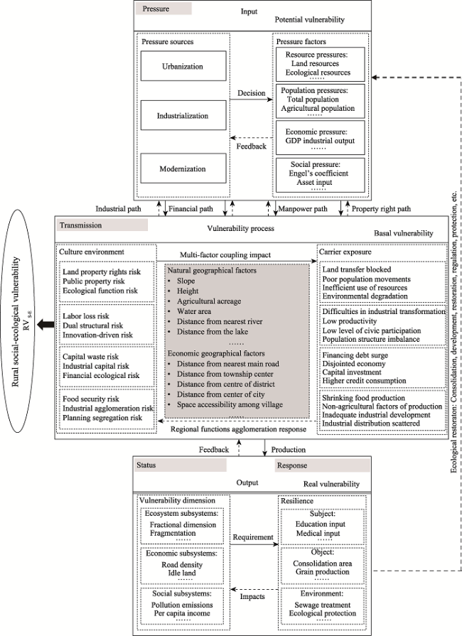
Fig. 1 The framework of rural social-ecosystem vulnerability |
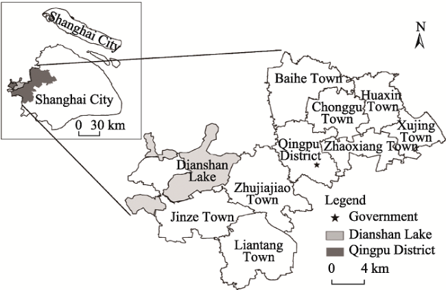
Fig. 2 Location of the case study area |
Table 1 Evaluation index system of social-ecosystem vulnerability in each administrative village in 2018 |
| Target | Criteria | Indicator | Indicator description and data source |
|---|---|---|---|
| Economic vulnerability | Pressure (Input) | Gross income of region (yuan) | The overall regional economic difference, using economic statistics data |
| Growth rate of secondary and tertiary industries (%) | The non-agriculture development difference, using economic statistics data | ||
| Total value of farm output (yuan) | The agriculture development difference, using rural statistics data | ||
| State (Output) | Per capita income (yuan person-1) | Individual resistance to vulnerability, using the household survey data | |
| Household income (yuan) | Family resilience to vulnerability, using the household survey data | ||
| Net household income (yuan) | Family resilience to vulnerability, using the household survey data | ||
| Response (Output) | Per capita disposable income (yuan person-1) | Family environment improvement capacity, using economic statistics data | |
| Road density (%) | Rural external communication capacity, using the land use vector data | ||
| Social vulnerability | Pressure (Input) | Urbanization rate (%) | Regional non-agricultural population pressure, using economic statistics data |
| Total population (person) | Regional population carrying pressure, using economic statistics data | ||
| Density of population (person km-2) | The per unit area population carrying pressure, using economic statistics data | ||
| State (Output) | Net population outflow (person) | State of social identity change, using the rural survey data | |
| Ratio of settled and farmland (%) | State ofhousehold livelihood capital, using the land use vector data | ||
| Number of agricultural workers (person) | Rural social employment, using the rural survey data | ||
| Deserted farmland area (ha) | State of agricultural behavior, using rural statistics data | ||
| Grain yield (t) | State of regional food security, using economic statistics data | ||
| Response (Output) | Fixed investments (yuan) | Resilience in social services, using economic statistics data | |
| Household education expenditure (yuan) | Family resilience to vulnerability, using the household survey data | ||
| Medical insurance coverage (%) | Resilience in public services, using economic statistics data | ||
| Ecological vulnerability | Pressure (Input) | Fertilizer usage (t) | Environmental pollution pressure of agriculture, using the rural survey data |
| Plastic film application (t) | Environmental pollution pressure of agriculture, using the rural survey data | ||
| Pollution emissions (t) | Industrial pollution pressure, using the environmental survey data | ||
| State (Output) | Vegetation coverage (%) | State of green land, using the land use vector data | |
| Land degradation index | State of regional land quality, using the land degradation classification data | ||
| Land patch density (piece ha-1) | State of land fragmentation, using the land use vector data | ||
| Agricultural landscape fractal dimension | State of agricultural shape, using the land use vector data | ||
| Response (Output) | Land consolidation area (ha) | Regional ecological improvement, using economic statistics data | |
| Environmental protection input (yuan) | Regional environmental protection efforts, using economic statistics data | ||
| Grain production per unit area (kg ha-1) | Regionalfood productivity, using economic statistics data |
Table 2 Geographical factors influencing social-ecosystem vulnerability of the administrative villages |
| Category | Indicator | Calculation method |
|---|---|---|
| Natural Geographical Attributes | Y1 Slope (%) | Slope data (resolution 30 m). Using DEM data extraction and re-classification: 0°-1°, 1°-2° and 2°-3° assigned to 1, 2, 3 |
| Y2 Elevation (m) | Elevation data (resolution 30 m). Using DEM data extraction | |
| Y3 Agricultural acreage (ha) | Extraction of arable land areas from land vector maps | |
| Y4 Water area (ha) | Extraction of water areas from land vector maps | |
| Y5 Distance from nearest river (km) | Using the river grid data extraction statistics. Grid vector layer (30 m*30 m), overlay administrative village committee and river grid layer, and use grid calculator statistics | |
| Y6 Distance from Dianshan Lake (km) | The calculation process was the same as above (Y5). Statistics from Village Committee to Dianshan Lake Center | |
| Economic Geographical Attributes | Y7 Distance from nearest main road (km) | The calculation process was the same as above (Y5). Statistics from Village Committee to the nearest main road |
| Y8 Distance from township center (km) | The calculation process was the same as above (Y5). Statistics from Village Committee to the nearest township center | |
| Y9 Distance from center of Qingpu District (km) | The calculation process was the same as above (Y5). Statistics from Village Committee to the Government of Qingpu District | |
| Y10 Distance from center of Shanghai City (km) | The calculation process was the same as above (Y5). Statistics from Village Committee to the Government of Shanghai City | |
| Y11 Space accessibility among village | The ‘grid calculator’ was used to calculate the minimum time cost of each grid after the superposition of the road grid layer and the ground grid layer The average value of all time costs associated with an administrative village were used as the index value of spatial accessibility of the village area |
Table 3 The comparison of vulnerability assessment for administrative villages in Qingpu District of 2018 |
| Region | CCR-DEA model | ACE-DEA model | EW-DEA model | |||
|---|---|---|---|---|---|---|
| Average of RVS-E | RVS-E | Average of RVS-E | RVS-E | Average of RVS-E | RVS-E | |
| Qingpu District | 0.623 | 0.699 | 0.583 | |||
| Eastern part | 0.689 | 0.756 | 0.625 | |||
| Central part | 0.542 | 0.643 | 0.554 | |||
| Western part | 0.638 | 0.699 | 0.609 | |||
| Guanglian Village in Xujing | 0.598 | 0.665 | 0.662 | |||
| Songshan Village in Huaxin | 7.125 | 7.193 | 7.194 | |||
| Chuiyao Village in Zhaoxiang | 0.629 | 0.698 | 0.703 | |||
| Zhongxin Village in Chonggu | 1.000 | 0.924 | 0.648 | |||
| Tangyu Village in Xiayang | 0.554 | 0.655 | 0.592 | |||
| Heqiao Village in Yingpu | 0.665 | 0.777 | 0.706 | |||
| Jinxing Village in Xianghuaqiao | 1.000 | 0.964 | 0.614 | |||
| Wangjing Village in Baihe | 1.000 | 0.972 | 0.729 | |||
| Wanlong Village in Zhujiajiao | 0.551 | 0.632 | 0.580 | |||
| Beidai Village in Liantang | 1.000 | 0.985 | 0.732 | |||
| Tianshanzhuag Village in Jinze | 0.582 | 0.676 | 0.626 | |||
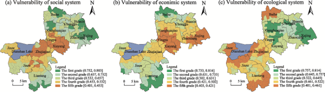
Fig. 3 Social-economic-ecosystem vulnerability in Qingpu District in the year 2018 |
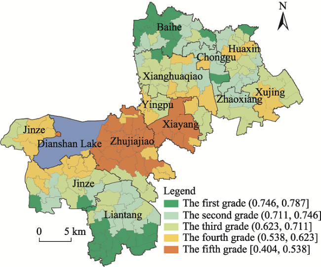
Fig. 4 Social-ecosystem vulnerability grades in Qingpu District in 2018 |
Table 4 The coupling results of vulnerability grades and influencing factors |
| Matching type | Y9 | Y6 | Y10 | Y4 | Y11 | Y7 | Y3 |
|---|---|---|---|---|---|---|---|
| -4 | 6.63 | 10.25 | 8.68 | 4.55 | 0.85 | 5.66 | 1.67 |
| -3 | 15.57 | 19.54 | 16.52 | 16.68 | 9.66 | 12.68 | 10.57 |
| -2 | 29.68 | 28.54 | 25.35 | 22.58 | 18.57 | 19.54 | 16.68 |
| -1 | 37.51 | 35.44 | 29.87 | 26.64 | 26.64 | 24.65 | 19.54 |
| 0 | 43.56 | 41.25 | 34.89 | 33.45 | 32.24 | 31.55 | 25.67 |
| 1 | 8.51 | 9.56 | 5.65 | 5.65 | 3.55 | 2.51 | 3.24 |
| 2 | 19.65 | 18.64 | 16.66 | 14.68 | 16.54 | 14.66 | 15.63 |
| 3 | 34.57 | 25.62 | 26.58 | 26.44 | 27.66 | 22.28 | 21.58 |
| 4 | 49.68 | 34.58 | 40.11 | 39.54 | 41.42 | 37.65 | 32.54 |
Note: Variable names are given in Table 2. |
Table 5 Coupling analysis of vulnerability grades and influencing factors |
| Region | Township | Y6 | Y7 | Y3 | Y11 | Y9 | Y4 | Y10 |
|---|---|---|---|---|---|---|---|---|
| Eastern part | Xujing | 0.446 | 0.269 | 0.115 | 0.329 | 0.584 | 0.326 | 0.358 |
| Zhaoxiang | 0.459 | 0.258 | 0.126 | 0.308 | 0.572 | 0.338 | 0.369 | |
| Huaxin | 0.449 | 0.246 | 0.175 | 0.215 | 0.569 | 0.345 | 0.372 | |
| Chonggu | 0.455 | 0.281 | 0.205 | 0.229 | 0.557 | 0.366 | 0.395 | |
| Baihe | 0.385 | 0.314 | 0.459 | 0.217 | 0.507 | 0.397 | 0.337 | |
| Central part | Xiayang | 0.315 | 0.210 | 0.511 | 0.262 | 0.451 | 0.401 | 0.468 |
| Xianghuaqiao | 0.324 | 0.235 | 0.469 | 0.259 | 0.449 | 0.386 | 0.459 | |
| Yingpu | 0.339 | 0.219 | 0.485 | 0.253 | 0.432 | 0.412 | 0.447 | |
| Western part | Zhujiajiao | 0.512 | 0.345 | 0.411 | 0.401 | 0.495 | 0.450 | 0.455 |
| Liantang | 0.499 | 0.348 | 0.109 | 0.354 | 0.502 | 0.259 | 0.451 | |
| Jinze | 0.642 | 0.195 | 0.516 | 0.358 | 0.265 | 0.491 | 0.311 | |
| Qingpu District | 0.475 | 0.304 | 0.284 | 0.331 | 0.532 | 0.394 | 0.428 | |
Note: Variable names are given in Table 2. |
Table 6 The coupling analysis of vulnerability grades and influencing factors |
| Region | Subsystem | Y6 | Y7 | Y3 | Y11 | Y9 | Y4 | Y10 |
|---|---|---|---|---|---|---|---|---|
| Eastern part | Social system | 0.387 | 0.259 | 0.188 | 0.169 | 0.511 | 0.115 | 0.438 |
| Economic system | 0.212 | 0.208 | 0.109 | 0.161 | 0.586 | 0.074 | 0.354 | |
| Ecological system | 0.145 | 0.186 | 0.125 | 0.175 | 0.689 | 0.106 | 0.341 | |
| Central part | Social system | 0.336 | 0.393 | 0.274 | 0.311 | 0.497 | 0.325 | 0.498 |
| Economic system | 0.301 | 0.328 | 0.227 | 0.264 | 0.457 | 0.247 | 0.468 | |
| Ecological system | 0.299 | 0.337 | 0.241 | 0.301 | 0.448 | 0.295 | 0.457 | |
| Western part | Social system | 0.454 | 0.232 | 0.438 | 0.194 | 0.396 | 0.428 | 0.404 |
| Economic system | 0.421 | 0.228 | 0.425 | 0.148 | 0.336 | 0.417 | 0.333 | |
| Ecological system | 0.409 | 0.214 | 0.412 | 0.186 | 0.298 | 0.398 | 0.347 | |
| Qingpu District | Social system | 0.396 | 0.279 | 0.267 | 0.235 | 0.435 | 0.279 | 0.413 |
| Economic system | 0.365 | 0.255 | 0.254 | 0.191 | 0.460 | 0.246 | 0.385 | |
| Ecological system | 0.381 | 0.246 | 0.259 | 0.221 | 0.478 | 0.266 | 0.382 |
Note: Variable names are given in Table 2. |
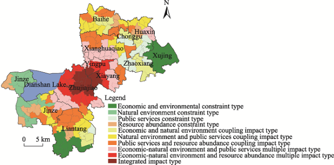
Fig. 5 The spatial distribution of coupling types of the geographical factors for social-ecosystem vulnerability in Qingpu District |
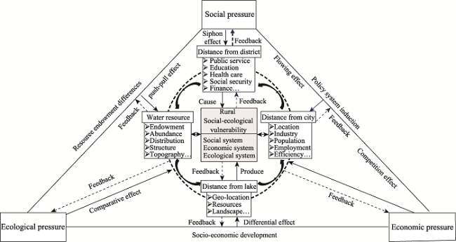
Fig. 6 The mechanism of geographical coupling for rural social-ecosystem vulnerability |
Table 7 The geographical impact types and ecological restoration modes of the social-ecosystem vulnerability in Qingpu District |
| Geographical impact types | Vulnerability characteristics | Governance emphases | Governance measures | Governance objects | Restoration modes |
|---|---|---|---|---|---|
| Economic environment constraint type | High grade of vulnerability High vulnerability of social and ecological systems Rapid loss of the rural population and rural culture dies out | Rural organization and culture | Comprehensive rural social improvement | √ Rural subject raise √ Rural order reconstruction | Embedded mode |
| Natural environment constraint type | Low grade of vulnerability High vulnerability of economic system Agricultural productivity and environmental pollution | Land resources | Agricultural land renovation | √ Cultivated land protection, capacity upgrade √ Leisure industry exploited | Consolidation mode |
| Public services constraint type | High grade of vulnerability High vulnerability of social and ecological systems Unequal coverage of public services | Social public spaces | Removing and reforming government | √ Multi-subject coordination √ Step-by-step promotion | Renew mode |
| Resource abundance constraint type | Medium grade of vulnerability High vulnerability of economic and ecological systems Water resources development and water pollution | Water pollution | Water Environment treatment | √ Node protection √ Sewage treatment | Oriented mode |
| Economic and natural environment coupling impact type | High grade of vulnerability High vulnerability of social and ecological systems Dilemma of industrial choice | Industrial types undertaken | Industrial renovation | √ Industrial upgrading √ Industrial chain extension | Cascaded mode |
| Natural environment and public services coupling impact type | High grade of vulnerability High vulnerability of social and economic system Public services extension | Public services integration | Infrastructure government | √ Convenient services √ Industrial and city emergent | Equivalent mode |
| Public services and resource abundance coupling impact type | High grade of vulnerability Medium vulnerability of all subsystems Public space accessibility and connectivity | Space fragmentation | Ecological remediation | √ Hydrophilic green bank √ Water-green blend | Dredging mode |
| Economic-natural environment and public services multiple impact type | High-low grade of vulnerability High social and ecological systems Vacant and wasteful resources | Resources use efficiency | Reduction government | √ Increase & decrease contact √ Intensive use | Displacement mode |
| Economic-natural environment and resource abundance multiple impact type | High-low grade of vulnerability High-low economic system Industrial structure rigid | Space quality | Environmental Improvement | √ Outskirt planning √ Ecotourism | Outskirt mode |
| Integrated impact type | Low grade of vulnerability Low vulnerability of all subsystems Coordinated development | Resources overall planning | Integrated territory consolidation | √ Urban and rural city emergent √ Integration | Aggregative model |
This research was supported by the Training of Young & Key Teachers in Higher Education Schools in Hunan Province.
| [1] |
|
| [2] |
|
| [3] |
|
| [4] |
|
| [5] |
|
| [6] |
|
| [7] |
|
| [8] |
|
| [9] |
|
| [10] |
|
| [11] |
|
| [12] |
|
| [13] |
|
| [14] |
IPCC. 2007. Summary for policymakers, fourth assessment report (AR4). New York, USA: Cambridge University Press: 1024-1085.
|
| [15] |
|
| [16] |
|
| [17] |
|
| [18] |
|
| [19] |
|
| [20] |
|
| [21] |
NBSC (National Bureau of Statistics of China). 2009-2019. China statistical yearbook. Beijing, China: Chinese Statistics Press.
|
| [22] |
|
| [23] |
|
| [24] |
|
| [25] |
|
| [26] |
|
| [27] |
|
| [28] |
|
| [29] |
|
| [30] |
|
| [31] |
|
| [32] |
|
| [33] |
|
/
| 〈 |
|
〉 |