
Journal of Resources and Ecology >
Predictability of Functional Diversity Depends on the Number of Traits
Received date: 2020-10-27
Accepted date: 2021-01-04
Online published: 2021-07-30
Supported by
The National Natural Science Foundation of China(31872683)
The National Natural Science Foundation of China(31800368)
The National Key Research and Development Program of China(2017YFA0604803)
Analysis of functional diversity, based on plant traits and community structure, provides a promising approach for exploration of the adaptive strategies of plants and the relationship between plant traits and ecosystem functioning. However, it is unclear how the number of plant traits included influences functional diversity, and whether or not there are quantitatively dependent traits. This information is fundamental to the correct use of functional diversity metrics. Here, we measured 34 traits of 366 plant species in nine forests from the tropical to boreal zones in China. These traits were used to calculate seven functional diversity metrics: functional richness (functional attribute diversity (FAD), modified FAD (MFAD), convex hull hypervolume (FRic)), functional evenness (FEve), and functional divergence (functional divergence (FDiv), functional dispersion (FDis), quadratic entropy (RaoQ)). Functional richness metrics increased with an increase in trait number, whereas the relationships between the trait divergence indexes (FDiv and FDis) and trait number were inconsistent. Four of the seven functional diversity indexes (FAD, MFAD, FRic, and RaoQ) were comparable with those in previous studies, showing predictable trends with a change in trait number. We verified our hypothesis that the number of traits strongly influences functional diversity. The relationships between these predictable functional diversity metrics and the number of traits facilitated the development of a standard protocol to enhance comparability across different studies. These findings can support integration of functional diversity index data from different studies at the site to the regional scale, and they focus attention on the influence of quantitative selection of traits on functional diversity analysis.
Key words: trait; functional diversity; richness; evenness; divergence; stability; predictability
ZHANG Zihao , HOU Jihua , HE Nianpeng . Predictability of Functional Diversity Depends on the Number of Traits[J]. Journal of Resources and Ecology, 2021 , 12(3) : 332 -345 . DOI: 10.5814/j.issn.1674-764x.2021.03.003
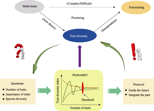
Fig. 1 The opportunities and challenges associated with functional diversity |
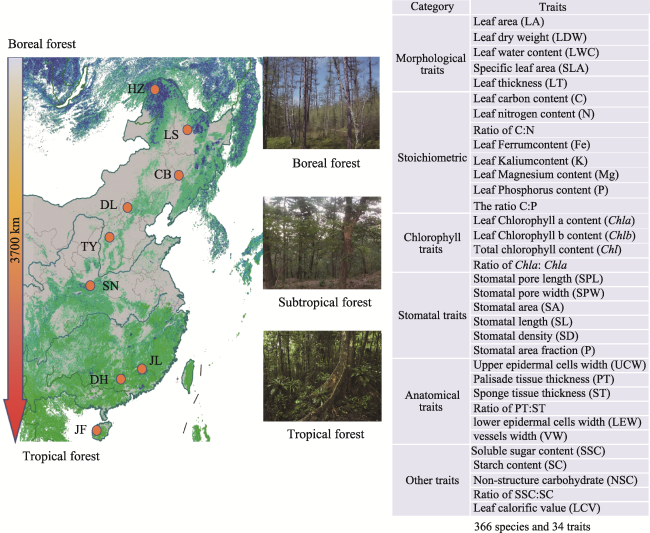
Fig. 2 The spatial distribution of nine forest communities from the boreal to the tropical zone in ChinaNote: A total of 34 functional traits and 366 species were sampled across the nine forest sites (orange circles). |
Table 1 The protocol of the functional diversity index |
| Functional diversity | Specific indexes | Description | Predictable | Fitted equation |
|---|---|---|---|---|
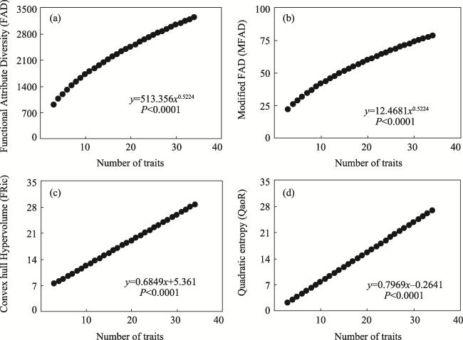
| Functional richness | Functional Attribute Diversity (FAD) | The sum of the distances of species in trait space | Yes | Y=513.356x0.5224† |
| Modified FAD (MFAD) | Modified FAD, includes species diversity | Yes | Y=12.4681x0.5224 | |
| Convex hull hypervolume (FRic) | Convex hull hypervolume | Yes | Y=0.6849x+5.3610 | |
| Functional evenness | Functional Evenness (FEve) | Distribution rule of trait space occupied by traits | No | |
| Functional divergence | Functional Divergence (FDiv) | Dispersion of functional traits | No | |
| Functional Dispersion (FDis) | Dispersion of functional traits | No | ||
| Rao's Quadratic entropy (RaoQ) | Both trait richness and trait dispersion | Yes | Y=0.7969x-0.2641 |
Note: † These prediction equations were reduced on all data of the nine forest communities from the tropical to the boreal zone. Detail information for each forest is presented in the supplementary files. |
Fig. 3 Relationship between functional diversity metrics and trait number different results. |
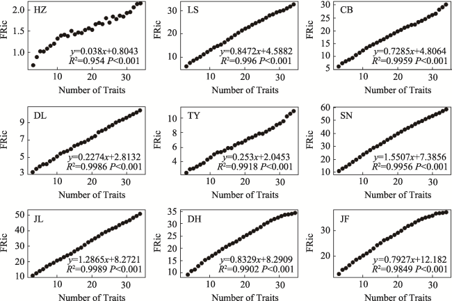
Fig. S1 The relationship between convex hull hypervolume (FRic) and the selected number of traits in different typical forestsNote: HZ, HuZhong; LS, LiangShui; CB, ChangBai; DL, DongLing; TY, TaiYue; SN, ShenNong; JL, JiuLian; DH, DingHu; JF, JianFengLing. |
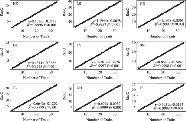
Fig. S2 The relationship between quadratic entropy (RaoQ) and the number of traits in different typical forestsNote: HZ, HuZhong; LS, LiangShui; CB, ChangBai; DL, DongLing; TY, TaiYue; SN, ShenNong; JL, JiuLian; DH, DingHu; JF, JianFengLing. |
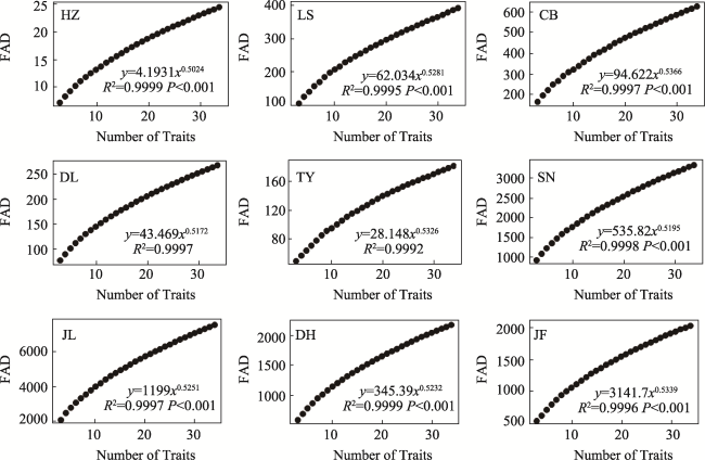
Fig. S3 The relationships between functional Attribute Diversity (FAD)and the number of traits in different typical forestsNote: HZ, HuZhong; LS, LiangShui; CB, ChangBai; DL, DongLing; TY, TaiYue; SN, ShenNong; JL, JiuLian; DH, DingHu; JF, JianFengLing. |
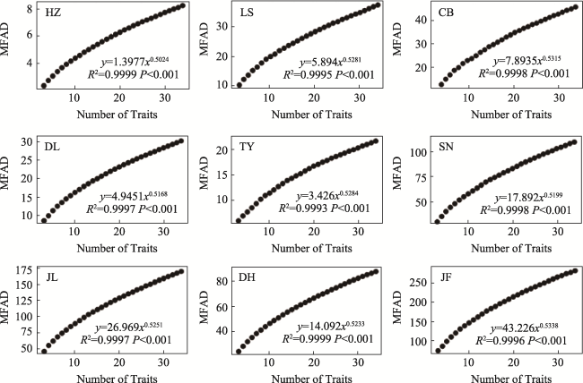
Fig. S4 The relationships between modified Functional Attribute Diversity (MFAD) and the number of traits in different typical forestsNote: HZ, HuZhong; LS, LiangShui; CB, ChangBai; DL, DongLing; TY, TaiYue; SN, ShenNong; JL, JiuLian; DH, DingHu; JF, JianFengLing. |
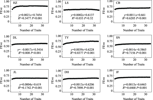
Fig. S5 The relationships between functional evenness (FEve) and the number of traits in different typical forestsNote: HZ, HuZhong; LS, LiangShui; CB, ChangBai; DL, DongLing; TY, TaiYue; SN, ShenNong; JL, JiuLian; DH, DingHu; JF, JianFengLing. |
Fig. S6 The relationship between functional divergence (FDiv) and the number of traits in different typical forestsNote: HZ, HuZhong; LS, LiangShui; CB, ChangBai; DL, DongLing; TY, TaiYue; SN, ShenNong; JL, JiuLian; DH, DingHu; JF, JianFengLing. |
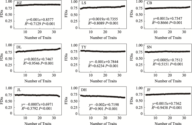
Fig. S7 The relationship between functional dispersion (FDis) and the number of traits in different typical forestsNote: HZ, HuZhong; LS, LiangShui; CB, ChangBai; DL, DongLing; TY, TaiYue; SN, ShenNong; JL, JiuLian; DH, DingHu; JF, JianFengLing. |
Table S1 The list of these selected traits and their abbreviations |
| Category | Traits | Unit | Abbreviation | Category | Traits | Unit | Abbreviation |
|---|---|---|---|---|---|---|---|
Morphological traits | Leaf area | cm2 | LA | Stomatal traits | Stomatal pore length | μm | PL |
| Leaf dry weight | g | LDW | Stomatal pore width | μm | PW | ||
| Leaf water content | % | LWC | Stomatal area | mm2 | SA | ||
| Specific leaf area | mm2 mg-1 | SLA | Stomatal length | μm | SL | ||
| Leaf thickness | mm | LT | Stomatal density pores per mm2 SD | ||||
Stoichiometric | Leaf carbon content | % | LCC | Stomatal area fraction | % | P | |
| Leaf nitrogen content | % | N | Anatomical traits | upper epidermal cells width | μm | UEW | |
| Ratio of C:N | NA | C/N | Palisade tissue thickness (PT) | μm | PT | ||
| Leaf Ferrum content | mg g-1 | Fe | Sponge tissue thickness (ST) | μm | ST | ||
| Leaf Kalium content | mg g-1 | K | Ratio of PT:ST | NA | PT/ST | ||
| Leaf Magnesium content | mg g-1 | Mg | lower epidermal cells width | μm | LEW | ||
| Leaf Phosphorus content | mg g-1 | P | vessels width | μm | VW | ||
| Ratio of C:P | NA | C/P | Other traits | Soluble sugar content (SSC) | mg g-1 | SSC | |
Chlorophyll traits | Leaf Chlorophyll a content | mg g-1 | Chl a | Starch content (SC) | mg g-1 | SC | |
| Leaf Chlorophyll b content | mg g-1 | Chl b | Non-structure carbohydrate | mg g-1 | NSC | ||
| Total chlorophyll content | mg g-1 | Chl | Ratio of SSC:SC | NA | SSC/SC | ||
| Ratio of Chla: Chlb | NA | Chl a/b | Leaf calorific value | kJ cm-2 | LCV | ||
Table S2 The predictive equations of trait richness index (FRic) prediction equations at different sites (mean ±SE) |
| Area | Site† | Fitted equation (y = kx + b) | k | R2 |
|---|---|---|---|---|
| Temperate zone | HZ | y = 0.038x + 0.8043 | 0.038±0 a‡ | 0.954 |
| LS | y = 0.8472x + 4.5882 | 0.8472±0.0587 b | 0.996 | |
| CB | y = 0.7285x + 4.8064 | 0.7285±0.2366 b | 0.9959 | |
| Subtropics | DL | y = 0.2274x + 2.8132 | 0.2274±0.0925 a | 0.9986 |
| TY | y = 0.253x + 2.0453 | 0.253±0.0956 a | 0.9918 | |
| SN | y = 1.5507x + 7.3856 | 1.5507±0.1718 c | 0.9956 | |
| Tropic | JL | y = 1.2865x + 8.2721 | 1.2865±0.2096 c | 0.9989 |
| DH | y = 0.8329x + 8.2909 | 0.8329±0.5388 b | 0.9902 | |
| JF | y = 0.7927x + 12.1820 | 0.7927±0.1592 b | 0.9849 |
Note: † HZ, HuZhong; LS, LiangShui; CB, ChangBai; DL, DangLing; TY, TaiYue; SN, ShenNong; JL, JiuLian; DH, DingHu; JF, JianFengLing. ‡ There is no significant difference between data with the same alphabet in each column (P < 0.01). |
Table S3 The predictive equations of quadratic entropy (RaoQ) at different sites (mean ±SE) |
| Area | Site† | Fitted equation (y = kx + b) | k | R2 |
|---|---|---|---|---|
| Temperate zone | HZ | y = 0.5036x + 0.2167 | 0.5036±0 ab‡ | 0.9996 |
| LS | y = 1.1944x - 0.8658 | 1.1944±0.1098 f | 0.9997 | |
| CB | y = 1.141x - 0.8301 | 1.141±0.2149 f | 0.9997 | |
| Subtropics | DL | y = 0.4314x - 0.0682 | 0.4314±0.0366 a | 0.9998 |
| TY | y = 0.9301x - 0.7576 | 0.9301±0.0862 e | 0.9997 | |
| SN | y = 0.8623x + 0.2462 | 0.8623±0.1035 de | 0.9998 | |
| Tropic | JL | y = 0.6646x - 0.1202 | 0.6646±0.1134 bc | 0.9999 |
| DH | y = 0.699x - 0.0952 | 0.699±0.0609 cd | 0.9999 | |
| JF | y = 0.7051x + 0.0154 | 0.7051±0.0433 cd | 0.9999 |
Note: † HZ, HuZhong; LS, LiangShui; CB, ChangBai; DL, DangLing; TY, TaiYue; SN, ShenNong; JL, JiuLian; DH, DingHu; JF, JianFengLing. ‡ There is no significant difference between data with the same alphabet in each column (P < 0.01). |
Table S4 The predictive equations of functional attribute diversity (FAD) at different sites (mean ± SE). |
| Area | Site† | Fitted equation (y = Axk) | k | R2 |
|---|---|---|---|---|
| Temperate zone | HZ | y = 4.1931x0.5024 | 0.5024±0 a‡ | 0.9999 |
| LS | y = 62.034x0.5281 | 0.5281±0.0075 bc | 0.9995 | |
| CB | y = 94.622x0.5366 | 0.5366±0.0063 c | 0.9997 | |
| Subtropics | DL | y = 43.469x0.5172 | 0.5172±0.0023 b | 0.9997 |
| TY | y = 28.148x0.5326 | 0.5326±0.0163 b | 0.9992 | |
| SN | y = 535.82x0.5195 | 0.5195±0.0050 b | 0.9998 | |
| Tropic | JL | y = 1199x0.5251 | 0.5251±0.0020 bc | 0.9997 |
| DH | y = 345.39x0.5232 | 0.5232±0.0018 bc | 0.9999 | |
| JF | y = 3141.7x0.5339 | 0.5339±0.0015 c | 0.9996 |
Note: † HZ, HuZhong; LS, LiangShui; CB, ChangBai; DL, DangLing; TY, TaiYue; SN, ShenNong; JL, JiuLian; DH, DingHu; JF, JianFengLing. ‡ There is no significant difference between data with the same alphabet in each column (P < 0.01). |
Table S5 The predictive equations of modified functional attribute diversity (MFAD) at different sites (mean ±SE) |
| Area | Site† | Fitted equation (y = Axk) | k | R2 |
|---|---|---|---|---|
| Temperate zone | HZ | y = 1.3977x0.5024 | 0.5024±0 a‡ | 0.9999 |
| LS | y = 5.894x0.5281 | 0.5281±0.0075 bc | 0.9995 | |
| CB | y = 7.8935x0.5315 | 0.5315±0.0063 c | 0.9998 | |
| Subtropics | DL | y = 4.9451x0.5168 | 0.5168±0.0023 b | 0.9997 |
| TY | y = 3.426x0.5284 | 0.5284±0.0163 b | 0.9993 | |
| SN | y = 17.892x0.5199 | 0.5199±0.0050 b | 0.9998 | |
| Tropic | JL | y = 26.969x0.5251 | 0.5251±0.0020 bc | 0.9997 |
| DH | y = 14.092x0.5233 | 0.5233±0.0018 bc | 0.9999 | |
| JF | y = 43.226x0.5338 | 0.5338±0.0015 c | 0.9996 |
Note: † HZ, HuZhong; LS, LiangShui; CB, ChangBai; DL, DangLing; TY, TaiYue; SN, ShenNong; JL, JiuLian; DH, DingHu; JF, JianFengLing. ‡ There is no significant difference between data with the same alphabet in each column (P < 0.01). |

| 1 |
|
| 2 |
|
| 3 |
|
| 4 |
|
| 5 |
|
| 6 |
|
| 7 |
|
| 8 |
|
| 9 |
|
| 10 |
|
| 11 |
|
| 12 |
|
| 13 |
|
| 14 |
|
| 15 |
|
| 16 |
|
| 17 |
|
| 18 |
|
| 19 |
|
| 20 |
|
| 21 |
|
| 22 |
|
| 23 |
|
| 24 |
|
| 25 |
|
| 26 |
|
| 27 |
|
| 28 |
|
| 29 |
|
| 30 |
|
| 31 |
|
| 32 |
|
| 33 |
|
| 34 |
|
| 35 |
|
| 36 |
|
| 37 |
|
| 38 |
|
| 39 |
|
| 40 |
|
| 41 |
|
| 42 |
|
| 43 |
|
| 44 |
|
| 45 |
|
| 46 |
|
| 47 |
|
| 48 |
|
| 49 |
|
| 50 |
|
| 51 |
|
| 52 |
|
| 53 |
|
| 54 |
|
| 55 |
|
| 56 |
|
| 57 |
|
/
| 〈 |
|
〉 |
