Ecosystem Services and Ecological Risks of Land Resource

Synergic Relationship between the Grain for Green Program and the Agricultural Eco-economic System in Ansai County based on the VAR model

  • LI Yue 1, 3 ,
  • WANG Jijun , 1, 2, * ,
  • HU Xiaoning , 4, * ,
  • ZHAO Xiaocui 1
Expand
  • 1. Institute of Soil and Water Conservation, Northwest A & F University, Yangling, Shaanxi 712100, China;
  • 2. Institute of Soil and Water Conservation, Chinese Academy of Sciences, Yangling, Shaanxi 712100, China
  • 3. Xi’an Polytechnic University, Xi’an 710048, China;
  • 4. College of Science, Northwest A&F University, Yangling, Shaanxi 712100, China
*: WANG Jijun, E-mail: ;
HU Xiaoning, E-mail:

Received date: 2020-05-26

  Accepted date: 2020-10-25

  Online published: 2021-05-30

Supported by

The National Key Research and Development Program(2016YFC0501707)

The National Natural Science Foundation of China(41571515)

The National Key Research and Development Program(2016YFC0503702)

Abstract

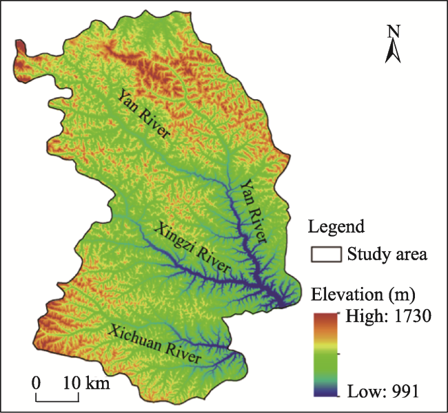
Understanding the synergic relationship between the Grain for Green Program (GGP) and the agricultural eco-economic system is important for designing an optimized agricultural eco-economic system and developing a highly efficient structure of an agricultural industry chain and a resource chain. This study used Ansai County time series data from 1995 to 2014, applied vector autoregressive (VAR) models and used tools such as Granger causality, impulse response analysis and variance decomposition, to explore the synergy between the GGP and the agricultural eco-economic system. The results revealed a synergic and reciprocal relationship between the GGP and the agroeconomic system. The contribution of the GGP to the agroecosystem reached 34%, which was significantly higher than either its largest contribution to the agroeconomic system (20.8%) or its peak contribution to the agrosocial system (26.7%). The agroeconomic system had the most prominent influence on the GGP, with a year-round stable contribution of up to 55.3%. These results were consistent with reality. However, the impact of the GGP on the agricultural eco-economic system was weaker than the effect of the agricultural eco-economic system on the GGP. The lag of variable stationarity after the shock was relatively short, indicating that optimal coupling had not formed between the GGP and the agricultural eco-economic system. On the basis of enhancing the ecological functions, we should construct the agricultural industry-resource chain such that it focuses on promoting the effective utilization of resources in the region. In addition, the development of a carbon sink industry can be used to manifest the ecological values of ecological functions.

Cite this article

LI Yue , WANG Jijun , HU Xiaoning , ZHAO Xiaocui . Synergic Relationship between the Grain for Green Program and the Agricultural Eco-economic System in Ansai County based on the VAR model[J]. Journal of Resources and Ecology, 2021 , 12(2) : 292 -301 . DOI: 10.5814/j.issn.1674-764x.2021.02.015

1 Introduction

In the past 20 years, the total budget of the Grain for Green Program (GGP), a landmark project for ecological restoration, reached 430 billion yuan (Bennett, 2008; Zinda et al., 2017). Statistics show the project has converted 2.98×10⁷ ha of farmland to forest and the average forest cover of the project areas increased by more than 3% (State Forestry Administration of the People’s Republic of China, 2016). Because of the scope, influence and duration of the program, it has become a focus of research for many scholars since its implementation.
A current research focus is the effect of the GGP on the agricultural eco-economic system of the former farming areas. Using rural household data in Ansai County in 2010, Li et al. (2016) established a model of structural equations and found that the implementation of the GGP had improved local farmers’ lives and promoted the transformation of local agriculture. However, this also led to the loss of local labor and arable land. Based on the monitoring data related to returning farmlands to forests, Chongqing historical yearbook data and past year environmental status bulletins, and field-involved household surveys, Gao et al. (2019) proved the project not only significantly improved vegetation coverage, but also played a positive role in soil and water conservation, such as by improving soil quality, purifying the atmosphere and sequestering carbon and releasing oxygen. Wang and Yue (2017) believed that after returning farmland to forest, the farmers’ income, including the subsidy for returning the farmland to forest, increased compared with that before the project was implemented so the project should be continued. Wang et al. (2014) used emergy to comprehensively examine the sustainable development of agricultural systems in the salt pond area in northwest China after the implementation of the GGP. The output of the agricultural systems in the study area increased from 1991 to 2008, but the increasing trend began to gradually decline after the GGP was implemented in 2001. According to the authors, this decline occurred mainly because the decreasing investment in nonrenewable resources reduced the effectiveness of the GGP and hindered the implementation of energy conservation and emission reduction policies. They suggested that the implementation of the GGP should be based on the effective use of low-carbon agricultural economy and the development of renewable resources. Lyu and Xu (2020) believed that these results suggest that the implementation of the GFG program would not induce an obvious risk to the food security. They also suggested that the GFG program should be set as a long-term strategic policy, not only by supporting the conversion of sloped farmlands, but also by helping local farmers to seek sustainable land use practices in order to improve their income and livelihood. Wang et al. (2015) modeled the coupling mechanism of a county-wide agro-ecological system and revealed that the ecological resources and agricultural production in the Loess hilly gully region did not match and coordinate with each other; in contrast, the GGP inhibited the ordered coupling of the agro-ecological system in the sample area. It is clear that the GGP not only brings great benefits to the ecological economy and society of rural areas through certain land subsidies, but also further promotes the development of systems such as farmer autonomy and farmer training (Gutiérrez et al., 2015; Li et al., 2018a). These researchers used a variety of methods to illustrate the effect of the GGP on the agro-ecological economy in the program areas from different perspectives. They also revealed that the GGP was affected by the development of the eco-economic systems in the program areas. However, the existing research has neither explicitly answered whether there is synergy between the GGP and the agricultural eco-economic system nor determined the potential intensity of the synergy. Therefore, this study focused on revealing and analyzing the synergy between the GGP and the agricultural eco-economic systems.
In the process of the abovementioned research, the main method used was comprehensive evaluation. However, these traditional static analysis methods fail to address the dynamic changes between systems and therefore have limitations in terms of revealing the synergy between the GGP and the agricultural eco-economic systems. To further reveal the existence of such a synergy, other research methods need to be explored. The vector autoregressive (VAR) model is a commonly used econometric model. Since its introduction by Sims in 1980 (Sims, 1980), it has quickly become a popular analytical tool for econometrics. VAR mainly replaced the simultaneous equations and improved the accuracy of economic forecasts. It uses linear or nonlinear regression analysis to combine theoretical analysis with practical statistics and determine the quantitative relationships between variables. The VAR model can analyze multiple economic indicators simultaneously. It is easy to estimate, has a good fit with data and is flexible and practical (Zhang, 2012). As the benchmark model of evaluation, the VAR model has been widely used in the fields of macroeconomic and financial forecasting. Therefore, the selection of VAR to analyze and study the synergy between the GGP and agricultural eco-economic systems is scientifically justified.
The county is the most basic unit in ecological engineering. A county has a moderate scale and clear boundaries. It is easy for operation and evaluation, is replicable and serves as a good scale for demonstration. In a county, the realization of plurality in the implementation of ecological projects is one of the effective approaches for exploring sustainable development in an area (Wang, 2018). As one of the pilot and representative counties of the GGP, the implementation of the program in Ansai County has brought observable agricultural, eco-economic and social benefits. Therefore, selecting Ansai County as the site to study the synergy between the GGP and the agricultural eco-economic system has a good scientific basis and representativeness.
Based on the background stated above, this article summarizes the descriptive statistics of agricultural, eco-economic and social data in the eight towns and three street areas in Ansai County for the period of 1995-2014. The agricultural, eco-economic and social development was analyzed before and after the implementation of GGP, and the results explicitly explained the synergy between the GGP and the development of the regional agricultural eco-economic system. The relationship between the GGP and the agricultural eco-economic system was also analyzed, which elucidated the synergy between the program and the agricultural eco-economic system in the program area, providing a reference for the coordinated development between the GGP and the agricultural eco-economic system.

2 Research area

Ansai County (108°51′44″-109°26′18″E, 36°30′45″-37°19′ 31″N) is located in the northern part of Yan’an City, Shaanxi Province. Its average elevation is 1371.9 m. The total area of the county is 2950 km2, accounting for 8.04% of the total area of Yan’an City, and the county has significant characteristics of a semi-arid and temperate continental monsoon climate, with four distinct seasons. With an average annual frost-free period of 160 days, average temperature of 9.1 ℃ and an average precipitation of 506.6 mm, this is a typical area of the Loess Plateau hilly gully region. According to statistics, the population of Ansai County was 197700 as of 2016, of which 151000 residents were active in agriculture. The county has cumulatively completed the national plan of forest restoration of 81747.52 ha. Of this total, 43328.32 ha (0.067 ha per farmer) were from retiring farmland, 36618.3 ha were from afforested land and wasteland restoration, and 1800.9 ha were from the conservation of existing forests. Since the implementation of the GGP, the area of soil erosion in the whole county has been reduced. The rate of erosion control reached 46%. The soil erosion module decreased from 14000 t km‒2 yr‒1 in 1998 to 5400 t km‒2 yr‒1 in 2014. The forest cover increased from 18% in 1998 to 34% in 2014. The per capita net income of farmers increased from 821 yuan in 1995 to 10,620 yuan in 2016.
Fig. 1 Overview of the study area

3 Research method and indicator extraction

3.1 Research method

In this study, the VAR model was used to analyze the reciprocal effect at the regional level. Christopher Sims proposed this approach in 1980. Compared to structural econometric models, the VAR model does not have any a priori constraints on the variables in the system and it makes all current variables apply regression on the lagged terms of all variables. This model avoids several complicated issues, such as the subjective division of endogenous variables and exogenous variables because of imperfect economic theories (Hosseini and Verma, 2017; Tiwari et al., 2019). The VAR method has a unique applicability to studying the dynamic interrelationships between a series of variables. Using four variables as an example, the model is expressed as follows (GGP, STXT, JJXT and SHXT are the Grain for Green Program, agroecosystem, agroeconomic system and agrosocial system, respectively):
$\begin{align} & \left[ \begin{matrix} GG{{P}_{t}} \\ STX{{T}_{t}} \\ JJX{{T}_{t}} \\ SHX{{T}_{t}} \\ \end{matrix} \right]=\left[ \begin{array}{*{35}{l}} {{c}_{1}} \\ {{c}_{2}} \\ {{c}_{3}} \\ {{c}_{4}} \\ \end{array} \right]+\left[ \begin{array}{*{35}{l}} a_{11}^{1}\text{ }a_{12}^{1}\text{ }a_{13}^{1}\text{ }a_{14}^{1} \\ a_{21}^{1}\text{ }a_{22}^{1}\text{ }a_{23}^{1}\text{ }a_{24}^{1} \\ a_{31}^{1}\text{ }a_{32}^{1}\text{ }a_{33}^{1}\text{ }a_{34}^{1} \\ a_{41}^{1}\text{ }a_{42}^{1}\text{ }a_{43}^{1}\text{ }a_{44}^{1} \\ \end{array} \right]\left[ \begin{array}{*{35}{l}} GG{{P}_{t-1}} \\ STX{{T}_{t-1}} \\ JJX{{T}_{t-1}} \\ SHX{{T}_{t-1}} \\ \end{array} \right]+\cdots + \\ & \begin{matrix} \begin{matrix} {} \\ \end{matrix} & {} & \begin{matrix} {} & {} \\ \end{matrix} \\ \end{matrix}\left[ \begin{array}{*{35}{l}} a_{11}^{p}\text{ }a_{12}^{p}\text{ }a_{13}^{p}\text{ }a_{14}^{p} \\ a_{21}^{p}\text{ }a_{22}^{p}\text{ }a_{23}^{p}\text{ }a_{24}^{p} \\ a_{31}^{p}\text{ }a_{32}^{p}\text{ }a_{33}^{p}\text{ }a_{34}^{p} \\ a_{41}^{p}\text{ }a_{42}^{p}\text{ }a_{43}^{p}\text{ }a_{44}^{p} \\ \end{array} \right]\left[ \begin{array}{*{35}{l}} GG{{P}_{t-p}} \\ STX{{T}_{t-p}} \\ JJX{{T}_{t-p}} \\ SHX{{T}_{t-p}} \\ \end{array} \right]+\left[ \begin{array}{*{35}{l}} {{e}_{1}} \\ {{e}_{2}} \\ {{e}_{3}} \\ {{e}_{4}} \\ \end{array} \right] \\ \end{align}$
where the vector ${{[GG{{P}_{t}},\ STX{{T}_{t}},\ JJX{{T}_{t}},\ SHX{{T}_{t}}]}^{\text{T}}}$ is the time series of 4×1 matrix. [c1, c2, c3, c4]T is a 4×1 constant vector, aij is a 4×4 parameter matrix to be evaluated (i=1, 2, 3, 4; j=1, 2, 3, 4), p is the model’s lag order and [e1, e2, e3, e4]T is a 4×1 random disturbance vector, which satisfies the covariance Cov(ei, ej)=0 (ij). Through the estimation of the model, it is possible to examine whether three variables are affected by the historical changes of each variable. Meanwhile, the estimation can also provide the degree of dynamic influence between variables within a certain lag period.
The VAR method is an attractive research tool because it does not rely on strict economic theories. Only two aspects need to be clarified in the modeling process. The first is to identify which variables are related and include all related variables in the VAR model. The second is to determine the lag period k to make the model reflect the majority of influence between the variables.

3.2 Indicator extraction and preliminary analysis

3.2.1 Selection of indicators
Based on the selection criteria of the existing research indicators (Wang et al., 2010; Li et al., 2018b), combined with the characteristics of the VAR model, this article mainly extracted the analysis indicators of the VAR model from the indicators mentioned above: GGP, STXT, JJXT and SHXT.
GGP indicators include organization and management (the degree of coordination between county, town and village administrations and the degree of implementation of relevant policies), as well as implementation (the structure of eco-economic forests, the survival rate of restored forests and grasses and the quality of restored forests (stands) and grasses).
Agroecosystem indicators include ecological conditions (e.g., rainfall, soil erosion module, percentage of irrigable area and ratio of forest to grass areas) and agricultural resources (land use structure of farming, forest and livestock, and proportion of fruit orchards).
Agroeconomic system indicators include industrial situation (ratio of agricultural labor to nonagricultural labor, commodity processing and storage rates, watershed agricultural industry chain and relationship to resources) and economic benefit (the contribution of industry and sideline income, commodity rate of agricultural products, per capita income, realization rate of food potential and agricultural output to investment ratio).
Agrosocial system indicators include social development (improvement of living conditions, improvement of production environment and update in value perceptions) and social stability (the Gini Index, level of satisfaction with life and sustainability potential).
3.2.2 Consistency test
The Eviews software makes an estimate of the VAR model by establishing VAR objects. Therefore, the VAR model does not focus on the testing of parameters, but mainly studies the patterns of dynamic changes between series.
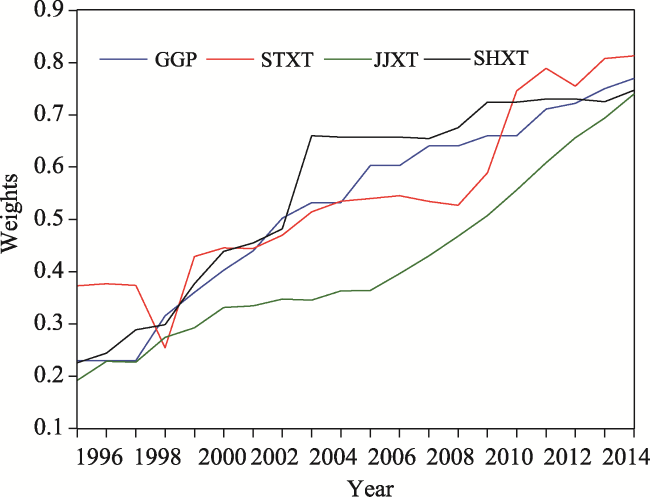
Fig. 2 Sequence diagram of the Grain for Green Program (GGP), agroecosystem, agroeconomic system, and agrosocial system. Note: “Weights” means the weights of Grain for Green Program and the agricultural eco-economic social system. GGP=Grain for Green Program, STXT=Agroecosystem, JJXT=Agroeconomic system, SHXT=Agrosocial system.
As shown in Fig. 2, the different variables in the series generally had a common trend, which allowed the construction of the VAR model.
3.2.3 Stability check
To eliminate the effects of heteroscedasticity to a certain extent and avoid the “pseudoresults” caused by direct analysis of time series, a stability check was needed for all series. The results of that test are shown in Fig. 3.
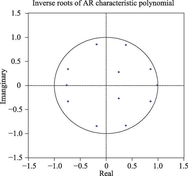
Fig. 3 VAR stability condition check
The characteristic root distribution was obtained by Eviews 8.0. The characteristic roots were all inside the unit circle, and the series was smooth. Therefore, the VAR model established in this study was stable.
3.2.4 Lag order determination
In addition to the stability condition that each data series needs to meet, the determination of the optimal lag order is another important part of the VAR model construction. In this article, the five criteria of LR, FPR, AIC, SC and HQ in Eviews software were used to study the optimal lag order selection of the VAR model. The results are shown in Table 1. When selecting the lag order identified as optimal by all five criteria, the VAR model could reasonably reflect the relationship between the GGP, agroecosystem, agroeconomic system and agrosocial system.
Table 1 Selection results of optimal lag orders
Lag ln L LR FPE AIC SC HQ
0 95.4200 NA 2.51E-10 ‒10.7553 ‒10.5593 ‒10.7358
1 162.4732 94.6633 6.63E-13 ‒16.7616 ‒15.7813 ‒16.6641
2 196.2529 31.7924 1.23E-13 ‒18.8533 ‒17.0888 ‒18.6779
3 268.7519 34.1172* 6.90E-16* ‒25.5002* ‒22.9516* ‒25.2469*

Note: * indicates the optimal lag order selected by each criterion; LR: sequential modified LR test statistic (each test at 5% level); FPE: Final prediction error; AIC: Akaike information criterion; SC: Schwarz information criterion; HQ: Hannan-Quinn information criterion; NA: Not Applicable.

Akaike information criterion (AIC) and Schwarz criterion (SC) were used to select the optimal lag order. Both criteria required their values to be as small as possible. When the optimal lag orders selected by the two criteria were not the same, the selection was made based on the results of the likelihood ratio (LR) test. Based on the principles stated above and the results shown in Table 1, the optimal lag order for the model was determined as 3.

4 Development and analysis of the VAR model

4.1 Granger causality test

Because the VAR model is unstructured and in a linear form, it is necessary to determine the interaction between variables and the maximum possible lag order of the interactions between reaction variables. Granger’s recommendation is to determine whether a variable's lag could cause a change in another variable. If a variable is influenced by the lag of other variables, then it can be assumed that there is Granger causality between them. Based on the VAR model, GGP, STXT, JJXT and SHXT were tested for Granger causality. The results are shown in Table 2.
As shown in Table 2, the P values were all less than 0.05, so the original hypothesis was rejected. This outcome indicated a strong two-way causal relationship between GGP and the agroecosystem, agroeconomic system and agrosocial system, and showed that the implementation of GGP had a great impact on these three systems. Simultaneously, changes in these systems also led to changes in the GGP.
Table 2 Results of Granger causality test
Excluded Chi-sq df Prob.
STXT is not a Granger cause of GGP 30.24180 3 0.0000
JJXT is not a Granger cause of GGP 14.37835 3 0.0024
SHXT is not a Granger cause of GGP 24.83216 3 0.0000
None of the three is a Granger cause of GGP 162.7878 9 0.0000
GGP is not a Granger cause of STXT 0.205770 3 0.0047
GGP is not a Granger cause of JJXT 13.55359 3 0.0036
GGP is not a Granger cause of STXT 24.04031 3 0.0000

4.2 Analysis of impulse response function

An impulse response function was carried out to comprehensively and intuitively reflect the dynamic influence of the change in one variable on the change of another variable. The impulse response function could reflect the amount of change in errors of the endogenous variables. By depicting these impact trajectories, it is possible to show how the perturbation of one variable affects the other variables through the model and ultimately feeds back to itself (Sims, 1972). In Figs. 4-6, the vertical axes are the response value, the horizontal axes are the number of lags of the impact, the dashed lines are two positive or negative standard deviations, and the solid lines represent the impulse response functions.
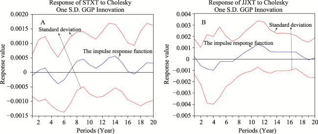
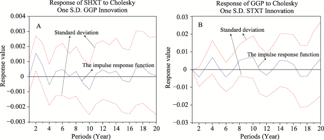
Fig. 4 (A) Impact of the impulse response function of the GGP impact on the agroecosystem and (B) Impact of the impulse response function of the GGP impact on the agroeconomic system
The analysis of the GGP impact response function on the ecosystem (Fig. 4A) shows that the forest restoration was only sporadic in the GGP areas before 1999. Therefore, the impact of GGP on the agroecosystem was not obvious in the first five periods. After the large-scale, official implementation of the GGP, the agroecosystem was optimized to some extent and presented an overall rising trend, increasing from ‒0.0001 in the first period to 0.00032 in the 20th period. This outcome indicated that the GGP had positive effects on the improvement of the ecosystem in the program area. The analysis of the GGP impact response function on the agroeconomic system (Fig. 4B) indicates that the GGP impact on the agroeconomic system of Ansai County started to show a rising trend after the 5th period. The impact shifted from negative to positive from the 8th period onward. In the 13th period, however, the impact of GGP on the agroeconomic system started to decline. This decline indicated that the increasing agricultural resources were not being utilized effectively with the advance of the GGP. The lack of structure in the industrial chain network reduced the effect of the GGP on the agroeconomic system, and that effect approached zero.
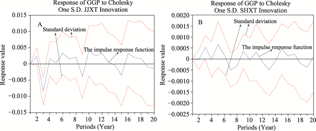
Fig. 5 (A) Impact of the impulse response function of the GGP on the agrosocial system and (B) impact of the impulse response function of the agroecosystem on GGP
The analysis of the response function of the GGP impact on the agrosocial system (Fig. 5A) showed that in the first few years of GGP implementation, the original production, lifestyle and consciousness had changed due to the large transfer of labor. The GGP had a positive impact on the agrosocial system. However, with the slowing down of program implementation, the social structure of Ansai began to rely more on the changes outside of the agricultural society. The impact of the GGP on the agrosocial system also decreased. By the 20th period, this impact was only 0.00023. According to the analysis of the response function of the ecosystem on the GGP (Fig. 5B), the impact of the agroecosystem on the GGP was always one period behind the impact of the GGP on the agroecosystem. This outcome indicated the existence of synergy between the GGP and the agroecosystem, which also shows a delay. Meanwhile, according to Fig. 5, the response rate of the impact of GGP on the agroecosystem was observably stronger than the response rate of the agroecosystem to the GGP. This outcome indicated that the ecosystem had a stronger impact on the GGP, which was consistent with the Granger test results.
The analysis of the agroeconomic system impact response function on the GGP (Fig. 6A) indicated a negative impact on the GGP in the early phase of the agroeconomic system. The impact shifted to mostly positive after the 4th period. The agroeconomic system had a negative impact on the GGP in the 3rd, 9th and 15th periods, corresponding to major natural disasters such as drought and hail. Since Ansai County had not yet completely shifted from traditional agriculture to modern agriculture, the productivity loss had a great impact on the development of the agricultural economy. The lagged development of the agricultural economy also produced a more obvious constraint on the implementation of the GGP. The analysis of the social system impact response function on the GGP (Fig. 6B) showed that the impact of the initial agrosocial system on the GGP was small. In general, the small response values indicated that the change in the agrosocial system in Ansai County had a very limited effect on the implementation of the GGP. Overall, because of the strong impact of the ecosystem on the GGP, these analysis results indicated that the impact of the GGP on the agricultural eco-economic system was less than the impact of the agricultural eco-economic system on the GGP.
Fig. 6 (A) Impact of the impulse response function of the agroeconomic system on GGP and (B) impact of the impulse response function of the agrosocial system on GGP

4.3 Variance decomposition

The impulse response function typically depicts a dynamic path of how one variable affects another. The variance decomposition can decompose the variables in the VAR model into individual disturbances. Using the horizontal structural changes to represent the changes of endogenous variables, the relative influence of each disturbance factor on each variable of the VAR model was provided. On this basis, the importance of structural impacts to variable changes was analyzed, and the sum of the individual contributions from all variables to the response variable was one. In this study, we analyzed the contributions of GGP, STXT, JJXT and SHXT to the changes of GGP, STXT, JJXT and SHXT, respectively. The analysis results are shown in Table 3-6. The rows represent the number of lagged periods (unit: year), and columns represent the contribution of each change in each period (%).
Table 3 Results of variance decomposition of GGP
Period GGP STXT JJXT SHXT
1 100.0000 0.000000 0.000000 0.000000
2 46.97864 0.275452 49.99727 2.748641
3 36.93287 0.189110 59.72816 3.149855
4 43.82030 5.560389 48.10528 2.514029
5 41.47807 6.651222 49.29604 2.574670
6 40.36725 7.864319 49.24901 2.519428
7 40.45021 7.857298 49.18690 2.505590
8 41.92192 7.802659 47.72272 2.552702
9 41.10650 7.647614 48.40435 2.841536
10 36.85136 6.952093 52.65719 3.539356
11 36.46208 6.884060 52.88802 3.765845
12 35.97839 6.968095 53.10793 3.945588
13 35.60862 6.868993 53.39047 4.131913
14 34.46051 6.724904 54.42927 4.385313
15 33.55404 6.487351 55.38504 4.573565
16 32.90078 6.334881 56.07234 4.691998
17 32.72247 6.247984 56.27963 4.749917
18 33.17266 6.238183 55.84694 4.742213
19 33.58538 6.178893 55.49491 4.740820
20 33.84172 6.066398 55.33573 4.756155
In Table 3, this disturbance dropped from the beginning of the 2nd period, and it started decreasing steadily by 30%-40% from the 4th period. The contributions of the agroecosystem, agroeconomic system and agrosocial systems to the GGP were each showing a gradual increasing trend. The response of the agricultural ecosystem to the impact of the GGP gradually started from the 3rd period, and was stable at approximately 6%-7% over the long-term. The response of the GGP to the impact of the agrosocial system was relatively small. It was 2.7% in the 2nd period and increased yearly thereafter. By the 20th period, the response had increased to 4.7%, which was consistent with the results of the impulse response analysis. Overall, in addition to the GGP’s self-disturbance, its largest contribution had come from the agroeconomic system. By the 20th period, the contribution reached as high as 55.33%. Simultaneously, the contributions of the economic system to the ecological and agrosocial systems had grown steadily since the 4th period and stabilized at 40%-70%. For example, the development of fruit trees and economic forests had been strengthened in terraced fields, land with gentle slopes, and other areas. This series of measures enabled the agroeconomic system in Ansai County to provide sufficient energy for the development of GGP.
Table 4 Results of variance decomposition of STXT
Period GGP STXT JJXT SHXT
1 34.03854 65.96146 0.000000 0.000000
2 24.16985 47.34999 26.74597 1.734188
3 22.66621 45.31722 29.97800 2.038576
4 23.87240 44.77885 29.48483 1.863920
5 20.98296 39.30572 37.74605 1.965261
6 21.01156 39.24508 37.71735 2.026013
7 18.12831 30.99178 47.64984 3.230058
8 16.21747 27.36007 52.56165 3.860810
9 16.48018 27.01160 52.57408 3.934142
10 16.88979 27.14635 52.10232 3.861549
11 17.20576 27.26732 51.69244 3.834473
12 18.57390 26.91517 50.71937 3.791569
13 18.39318 25.52646 52.21594 3.864421
14 18.18169 25.01597 52.90871 3.893628
15 18.16849 24.98703 52.95221 3.892270
16 18.02933 24.71425 53.35900 3.897418
17 18.48797 24.60392 53.03599 3.872119
18 19.04771 24.21242 52.86298 3.876884
19 19.06914 23.86512 53.14646 3.919277
20 19.02169 23.94952 53.09804 3.930749
In Table 4, during the 1st period, the contribution of the GGP to the agroecosystem was as high as 34%. Thereafter, the contribution declined over the years and started increasing from the beginning of the 11th period. This outcome was consistent with the progress of the GGP. At the beginning of the program, the implementation was more powerful. Farmland which was unsuitable for farming could be restored as forest within a short period of time. However, with the reduction of the program area, the contribution of the GGP to the ecosystem also gradually declined.
Table 5 Results of variance decomposition of JJXT
Period GGP STXT JJXT SHXT
1 1.182166 31.04439 67.77345 0.000000
2 10.99956 21.93295 58.37821 8.689267
3 11.62723 29.13453 45.50244 13.73580
4 6.480872 11.59514 67.78314 14.14085
5 4.166707 7.265975 73.83517 14.73215
6 3.222419 5.346392 76.93101 14.50018
7 2.470198 4.137165 79.50457 13.88807
8 2.786844 3.767963 80.35815 13.08704
9 4.136604 3.577964 79.91008 12.37535
10 5.712280 3.458045 78.95150 11.87818
11 7.744052 3.304099 77.51841 11.43344
12 11.05443 3.362066 74.66244 10.92106
13 13.87833 3.315876 72.26145 10.54434
14 16.14107 3.224412 70.37941 10.25511
15 17.99782 3.146222 68.82362 10.03234
16 19.33046 3.086780 67.69297 9.889791
17 20.01023 3.068669 67.07638 9.844721
18 20.33374 3.048619 66.75265 9.864993
19 20.44495 2.996728 66.62714 9.931181
20 20.27283 2.931656 66.76228 10.03323
In Table 5, the contribution of the GGP to the agroeconomic system increased from 1.19% in the 1st period to 20.28% in the 20th period, and fell to 2.47% in the 7th period. This outcome showed that in the early stage of the GGP, the program subsidy was relatively high, which had some effect on the economic income of the farmers in the program. However, due to the failure to fundamentally solve the problems in the industrial structure and resource allocation, the contribution of the program to the agricultural economic system dropped to its lowest value. After that, with the continuous optimization of the system and the adjustment of the industrial structure, the contribution of the program to the agroeconomic system began to steadily increase.
In Table 6, the contribution of the GGP to the agrosocial system devreased from 26.77% in the 2nd period to 25.5% in the 20th period. Thus, its contribution was relatively stable. These results indicate that the development of the agrosocial system relies more on the renewal of the external system, while the agrosocial system based on the GGP develops more slowly.
Table 6 Results of variance decomposition of SHXT
Period GGP STXT JJXT SHXT
1 18.87098 6.760140 70.84797 3.520917
2 26.76893 9.248055 60.95672 3.026292
3 27.11706 14.34652 55.47644 3.059981
4 25.22953 14.47205 56.99748 3.300943
5 27.17946 15.90058 53.79811 3.121845
6 28.83369 15.67092 52.44756 3.047826
7 28.17519 15.86272 52.85195 3.110131
8 27.65035 15.82999 53.31729 3.202368
9 27.11451 15.50274 54.21229 3.170458
10 27.29663 15.57717 54.00622 3.119978
11 26.90601 15.32391 54.48380 3.286285
12 25.86527 14.93348 55.65069 3.550558
13 25.11885 14.50791 56.65721 3.716026
14 25.24391 14.68999 56.33951 3.726583
15 25.23326 14.68276 56.34445 3.739534
16 25.51067 14.83210 55.93534 3.721885
17 25.55084 14.69503 56.01712 3.737012
18 25.41625 14.43714 56.38646 3.760148
19 25.49555 14.37880 56.36660 3.759053
20 25.49843 14.36618 56.37778 3.757611

5 Policy recommendations and conclusions

5.1 Policy recommendations

(1) The formulation and adjustment of the GGP policy should not only emphasize the goal of ecological restoration but also consider the ecological, economic and social sustainable development goals. (I) On the basis of ensuring the current scale of the GGP, the ecological functions should be improved through the adjustment of forest structure and the continuous optimization of biological communities. The relevant policy should be formulated with the goal of combining the sustainable use of ecological resources and the sustainable development of the agricultural economy. (II) Based on the principle of suitability, the restoration of ecological forests, the transformation of economic forests and the development of gently sloped land should be unified. The directions and focuses of the GGP need to be constantly adjusted. (III) The GGP should be combined with precision poverty relief to accelerate the alleviation of poverty during the restoration of regional ecology.
(2) The economic manifestation of the ecological functions should be promoted after the implementation of the GGP to improve the added value of ecological (agricultural) resources. The large amount of forest and grassland resources in Ansai County as the result of the GGP can be commercialized through carbon sinks to improve the added value of ecological resources (Silver et al., 2000; Jindal et al., 2008; Wei et al., 2015). This approach can then provide a breakthrough and a new growth point for the rearrangement of the original industrial structure and forest and grassland resources. Simultaneously, by taking advantage of that opportunity, a network structure of the agricultural industry chain can be built with the focus of improving the proportion of forest and grass resources to provide a solid material foundation for the coordinated development of the GGP and the agricultural eco-economic system, and promote the sustainable development of the program area.

5.2 Conclusions

Using the VAR model, this study analyzed the data from 1995 to 2014 for Ansai County and revealed the synergy between the GGP and the agricultural eco-economic system.
(1) The GGP not only had an impact on the agricultural eco-economic system but also had been reflexively influenced by the change in the agricultural eco-economic system. This outcome clearly verified the synergy between the two. The GGP and the agricultural eco-economic social system were the Granger causes of each other, which indicated that the implementation of the GGP promoted the agricultural, eco-economic and social development. Simultaneously, the continuous optimization of the agricultural eco-economic system in the region also had impacts on the GGP and promoted the adjustment and optimization of its policies.
(2) In general, the positive interactions between the GGP, the agroecosystem, agroeconomic system and agrosocial system were stronger than the negative interactions; however, the influence periods and intensities varied. The response of the GGP to the impact from the agricultural economic system was relatively strong. The reason might be that the original model of agricultural resource allocation was broken in the early stage of the GGP. The readjustment of industrial structure had also produced different positive and negative influences on the GGP. With the exception that the impact from the GGP on the agroeconomic system remained stable from the 9th period to the 17th period, the lagged stable states of the other variables after impact were all relatively short. The restoration and improvement of the agroecosystem in Ansai County were also influenced by other factors and disturbances in addition to the GGP.
(3) The GGP, agroecosystem, agroeconomic system and agrosocial system were greatly affected by their own changes in the early stages. Later, the influences of other variables gradually increased, taking up certain proportions and gradually stabilizing. The agricultural economic system contributed greatly to the GGP, the agroecosystem and the agrosocial system. This contribution showed that the GGP in Ansai County and the sustainable development in the area relied more heavily on the development of the agricultural economic system in the area. The impact of the GGP on the agroeconomic system was weaker than the impact of the agroeconomic system on the GGP. This outcome indicated that the GGP played an important role in the optimization of policies, which produced an internal driving force within the agroeconomic system and accelerated sustainable development in the GGP area.
1
Bennett M T . 2008. China’s sloping land conversion program: Institutional innovation or business as usual? Ecological Economics, 65(4): 699‒711.

2
Gao L, Yang X K, Hu H Z , et al. 2019. Analysis on ecological and economic benefits of implementing the Project of Returning Farmlands to Forests in Chongqing City. Research of Soil and Water Conservation, 26(6): 353‒358. (in Chinese)

3
Gutiérrez R L, Hogarth N J, Zhou W , et al. 2016. China’s conversion of cropland to forest program: A systematic review of the environmental and socioeconomic effects. Environmental Evidence, 5:21. DOI: 10.1186/s13750-016-0071-x.

4
Hosseini S D, Verma M . 2017. A Value-at-Risk (VAR) approach to routing rail hazmat shipments. Transportation Research Part D: Transport and Environment, 54(7): 191‒211.

5
Jindal R, Swallow B, Kerr J . 2008. Forestry-based carbon sequestration projects in Africa: Potential benefits and challenges. Natural Resources Forum, 32(2):116‒130.

6
Li Q R, Amjath-Babu T S, Sieber S , et al. 2018a. Assessing divergent consequences of payments for ecosystem serviceson rural livelihoods: A case-study in China’s Loess Hills. Land Degradation & Development, 29(10): 3549‒3570.

7
Li Q R, Liu Z, Zander P , et al. 2016. Does farmland conversion improve or impair household livelihood in smallholder agriculture system? A case study of Grain for Green Project impacts in China’s Loess Plateau. World Development Perspectives, 2: 43‒54.

8
Li Y, Wang J J, Liu P L , et al. 2018b. Study on the synergic relationship between grain for green and agricultural eco-economic social system—A case study in Ansai County. Journal of Natural Resources, 33(7): 1179‒1190. (in Chinese)

9
Lyu C H, Xu Z Y . 2020. Crop production changes and the impact of Grain for Green Program in the Loess Plateau of China. Journal of Arid Land. 12(1): 18‒28.

10
National Forestry and Grassland Administration of China. 2017. China forestry development report(2016). Beijing, China: China Forestry Publishing House. (in Chinese?)

11
Silver W L, Ostertag R, Lugo A E . 2000. The potential for carbon sequestration through reforestation of abandoned tropical agricultural and pasture lands. Restoration Ecology, 8(4): 394‒407.

12
Sims C A . 1972. Money, income, and causality. American Economic Review, 62(4): 540‒552.

13
Sims C A . 1980. Macroeconomics and reality. Econometrica, 48(1):1-48.

14
Tiwari A K, Cai Y F, Chang T . 2019. Monetary shocks to macroeconomic variables in China using time-vary VAR model. Applied Economics Letters, 26(20): 1664‒1669.

15
Wang J J, Guo M C, Jiang Z D , et al. 2010. The construction and application of an agricultural ecological-economic system coupled process model. Acta Ecologica Sinica, 30(9): 2371‒2378. (in Chinese)

16
Wang S, Yue X M . 2017. The Grain-for-Green Project, non-farm employment, and the growth of farmer income. Economic Research Journal, 52(4): 106‒119.

17
Wang X H, Shen J X, Zhang W . 2014. Emergy evaluation of agricultural sustainability of Northwest China before and after the Grain-for-Green Policy. Energy Policy, 67: 508‒516.

18
Wang Y J, Jiang Z D, Wang J J . 2015. Impact of sloping land conversion program on coupling of agricultural ecological system. Systems Engineering — Theory & Practice, 35(12): 3155‒3163.(in Chinese)

19
Wang Y. 2018. Green development strategy and challenges in agriculture.http://www.h2ochina.com/news/282165.html. [2019-02-15].

20
Wei X H, Zheng J, Liu G H , et al. 2015. The concept and application of carbon sequestration potentials in plantation forests. Acta Ecologica Sinica, 35(12):3881-3885. (in Chinese)

21
Zhang Y Q . 2012. On the identification issues of the structural VAR models: A review. Journal of Applied Statistics and Management, 31(5): 805‒812. (in Chinese)

22
Zinda J A, Trac C J, Zhai D L , et al. 2017. Dual-function forests in the returning farmland to forest program and the flexibility of environmental policy in China. Geoforum, 78: 119‒132.

Outlines

/