Land Use Change and Land Multifunction Tradeoffs

Damage or Recovery? Assessing Ecological Land Change and Its Driving Factors: A Case of the Yangtze River Economic Belt, China

  • ZHOU Ting 1 ,
  • QI Jialing 1 ,
  • XU Zhihan 2 ,
  • ZHOU De , 1, *
Expand
  • 1. Department of Land Resources Management, Zhejiang Gongshang University, Hangzhou 310000, China
  • 2. Land Consolidation and Rehabilitation Center of Zhejiang Province, Hangzhou 310007, China
*, ZHOU De, E-mail:

Received date: 2020-09-24

  Accepted date: 2020-11-30

  Online published: 2021-05-30

Supported by

The National Social Science Fund of China(19BGL283)

The National Natural Science Foundation of China(41301619)

Abstract

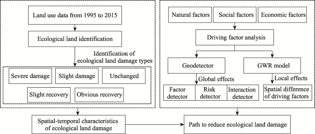
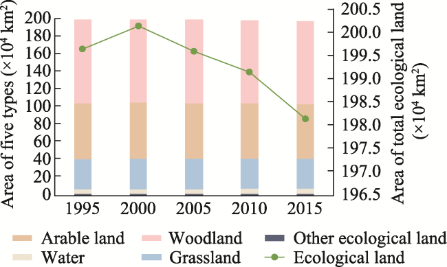
Ecological land can provide people with ecological products and ecological services; and it plays an important role in maintaining the health and safety of the ecosystem. With China’s rapid urbanization development, ecological land has been invaded in large quantities, and damaged seriously, even resulting in loses of its ecological function. Based on land use data from 1995 to 2015, our study explores the spatial and temporal evolution of the damage or recovery of ecological land in the Yangtze River Economic Belt (YREB). Two spatial models, geographic detector and geographic weighted regression (GWR), were employed to assess the global effects and the local effects of the driving factors for ecological land change, respectively. Our study divided the ecological land change into five types based on the degree of change as severe damage, slight damage, unchanged, slight recovery, and obvious recovery. The results show that from 1995 to 2015, the total area of ecological land in the YREB increased initially and then decreased, but the overall trend was decreasing. The total damaged area was larger than the recovered area. Arable land and woodland both showed downward trends. In terms of ecological land change over the past 20 years, the type of unchanged had the largest area, followed by slight damage and slight recovery. Our study further revealed that ecological land change was the net result of the interaction of many factors, and the explanatory power between any two driving factors was greater than that of any individual driving factor. In addition, driving factors have different impacts on ecological land change in different geographical locations. This knowledge should help land managers and policymakers to be better informed when developing pertinent land use policies at the regional and local levels. The lessons can also be extended to other regions for better management of their ecological land for sustainable use.

Cite this article

ZHOU Ting , QI Jialing , XU Zhihan , ZHOU De . Damage or Recovery? Assessing Ecological Land Change and Its Driving Factors: A Case of the Yangtze River Economic Belt, China[J]. Journal of Resources and Ecology, 2021 , 12(2) : 175 -191 . DOI: 10.5814/j.issn.1674-764x.2021.02.005

1 Introduction

Ecological land is one of the key resources and environments that people rely on for their survival. Ecological land can provide people with ecological products, ecological services, and ecological functions such as water conservation, soil protection, wind and sand fixation, climate regulation, environmental purification, and biodiversity protection (Yu et al., 2015). It plays an important role in maintaining the health and safety of the ecosystem (Costanza and Daly, 1992; Belmeziti et al., 2018).
Since China’s economic reform in 1978, its economy and urbanization have developed rapidly; while the expansion of cities has accelerated, and human interference and damage to the ecological environment have gradually increased (Tan et al., 2016). These developments have resulted in large amounts of ecological land becoming occupied and the loss of ecological functions, making the ecosystem more fragile, and ultimately causing many ecological and environmental problems. Therefore, understanding the extent of damage and spatial distribution of ecological land, and further exploring their driving factors are of great significance to the protection and scientific management of ecological land.
Previous studies on ecological land have mainly focused on connotation and classification (Rowe and Sheard, 1981; Klijn and Haes, 1994; Bajzak and Roberts, 1996; Bruce and Randal, 1996; Dong et al., 1999; Xiao et al., 2002; Zhang et al., 2004; Deng et al., 2009; Grondin et al., 2014), dynamic changes (Liu and Zhang, 2016; Li et al., 2017; Li et al., 2020), spatial patterns (Zhou et al., 2015; Zhu et al., 2015; Zhou et al., 2016; Zhang et al, 2017b), driving factors (Costanza et al., 1997; Xie et al., 2001; Xie and Li, 2011; Xie et al., 2013; Tang et al., 2016; Peng et al., 2017; Liu et al., 2020; Zhang et al., 2020), and ecosystem evaluation (Xiao and Li, 1997; Kathleen et al., 2013; Jozi and Majd, 2015; Peng et al., 2015; Yu et al., 2015; Naser et al., 2016; Liu et al., 2017; Jiang et al., 2019). In China, the term “ecological land” was first proposed by Dong et al. (1999), who defined the space of ecological elements as ecological land. Zhang et al. (2004) and Deng et al. (2009) discussed the concept of ecological land from different perspectives. Zhang et al. (2004) clarified the concept of ecological land in the arid area of Northwest China, and divided ecological land into artificial and natural types according to the land’s function. Deng et al. (2009) believed that ecological land refers to the land use type mainly regarding its ability to provide ecosystem services. In terms of the classification of ecological land, Bajzak and Roberts (1996) and Xiao et al. (2002) combined RS and GIS technology to classify and map ecological land. Bruce et al. (1996) and Pierre et al (2014) constructed a framework for studying the classification of ecological land. In this study, we combined the connotation of ecological land with the structure and function of the land use system, and considered its land use type and ecological service function.
The spatial pattern of ecological land and its driving factors have been studied by some scholars, such as Zhou et al. (2015), Zhu et al. (2015), Liu and Zhang (2016), Zhang et al. (2016), Zhou et al. (2016), and Li et al. (2020). The results have shown the importance of understanding the spatial characteristics of ecological land for better ecological land protection. On the basis of understanding the spatial pattern, scholars have further explored the driving factors that affect the change of ecological land. Many have used regression models to study driving factors. Xie and Li (2011), Xie et al. (2013) and Peng et al. (2017) analyzed the influencing factors of regional ecological land evolution based on a logistic regression model; Liu et al. (2020) explored the factors influencing ecological land based on a geographically weighted regression model in Wuhan urban agglomeration. As for the driving factors, different scholars have their own emphases. For example, Zheng et al. (2019) only considered the policy factors. Tang et al. (2016) studied various types of driving factors including natural factors, socio-economic factors, and mining (coal) resources based on reconstructed data; while Zhang et al. (2020) also considered natural factors and socio-economic factors.
In terms of ecological land evaluation, some scholars have carried out various forms of empirical analysis, including the assessment of ecosystem’s structures, functions, and service values. Xiao and Li (1997) combined ecological land with landscape ecology to carry out a study on landscape evaluation, management and ecological space planning. Liu et al. (2017a) combined it with landscape ecology theory to conduct an evaluation of ecological land fragmentation. Jozi and Majd (2015) carried out a capacity evaluation of ecological land to promote eco-tourism. Naser et al. (2016) combined RS and GIS technology to evaluate the suitability of ecological land. Jiang et al. (2019) evaluated urban ecological land use efficiency to protect the structure and function of the ecosystem, and enhance the ecological environment’s ability to support the development of the social environment. In addition, some scholars have introduced the concept of resource bearing capacity to study the ecological space occupation of natural resources (Xie et al., 2001). In recent years, there have been many studies on ecological land demand (Peng et al., 2015) and ecosystem service value estimation (Costanza, 1997; Kathleen et al., 2013; Yu et al., 2015).
Although the existing studies have made considerable achievements on this topic, they still have certain limitations. First, previous studies rarely assessed the extent of ecological land changes and identified their types. Second, in terms of the analysis of influencing factors, most existing studies used only a global model to explore the driving factors for ecological land at the global level, whereas they rarely assessed the effects of the driving factors at the local level.
At present, the Chinese government has begun to pay close attention to ecological environmental protection. China has not only promulgated relevant laws one after another, but also proposed the concept of an “ecological protection red line”, and emphasized the need to establish an ecological civilization concept that respects nature, conforms to nature, and protects nature (Hu, 2012). In addition, the “Outline of the master plan for national land use (2006-2020)” proposed to control production land, guarantee living land, and increase the proportion of ecological land; and this Plan also highlighted the need to improve the spatial structure of ecological land, to strictly protect the basic ecological land, and to build a sound ecological land use pattern. The Yangtze River Economic Belt (YREB) is a pioneering demonstration belt for the construction of the ecological civilization in China. Based on the guidance of the ecological priority and green development, the State Council highlighted that the YREB should strengthen the high-quality development and the coordinated development of the upper, middle and lower reaches of the Yangtze River.
Therefore, the purpose of this study is to understand the spatial-temporal evolution of ecological land change and its driving factors in the YREB based on five periods of land use data from 1995 to 2015. The specific aims of this paper are: (1) to identify the types of ecological land changes; (2) to assess the extent of ecological land change and the spatial differences; (3) to analyze the global effects and local effects of the driving factors on ecological land change by using geographic detector and geographically weighted regression (GWR) models.
This paper is organized as follows: Section 2 introduces the general situation of the study area; Section 3 describes the materials and methods used; Section 4 presents the findings of our study; Section 5 proposes ways to reduce the damage of ecological land and some limitations of our paper; and the conclusions are given in Section 6. The technical flowchart of this study is shown in Fig. 1.
Fig. 1 The technical flowchart of this study

2 Study area

The YREB straddles three major regions of China’s east, middle and west, and mainly covers 11 provincial regions and 130 cities (Fig. 2). The total area is about 2.05×10⁶ km2, accounting for 21.40 % of China. The upstream area of the Yangtze River includes Chongqing, Sichuan, Guizhou, and Yunnan, covering an area of about 1.137×10⁶ km2, accounting for 55.40 % of the YREB; while the midstream area includes Jiangxi, Hubei, and Hunan, with an area of about 5.646×10⁵ km2, accounting for 27.50 % of the YREB; and the downstream area includes Shanghai, Jiangsu, Zhejiang, and Anhui, covering an area of about 3.503×10⁵ km2, accounting for 17.10 % of the YREB. The region has a variety of topographic features and landforms such as hills, plains, and mountains, as well as many lakes such as the Yangtze River, Dongting Lake, and Poyang Lake (Chen, 2015).
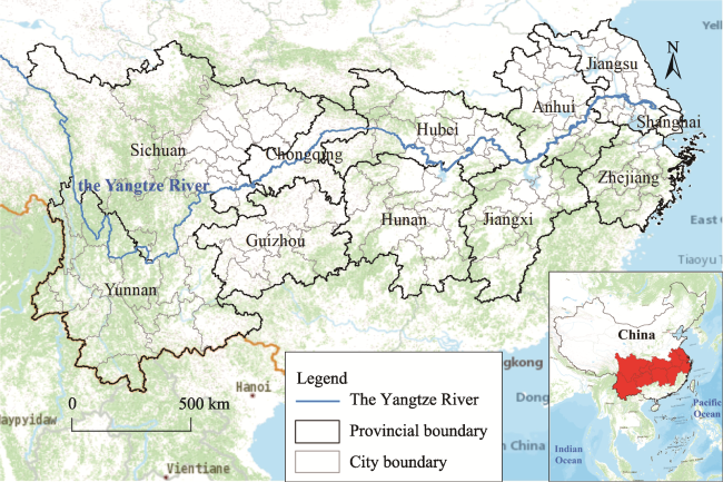
Fig. 2 Geographical location of the YREB
The YREB is a giant economic belt that spans various types of regions in the east, middle and west of China. It is also the most populous, the largest industrial, and the most complete river basin economic belt in China. It plays an important strategic role in the national economic development and the new urbanization development (Fang et al., 2015). In the past 25 years, the total GDP of the YREB has increased from 2.375×10¹² yuan in 1995 to 4.030×10¹³ yuan in 2018, accounting for 44.80 % of the China’s GDP in 2018. The total population of the YREB also increased, from 537 million in 1995 to 599 million in 2018, of which the urban population reached 356 million, accounting for 59.43 % of the total population in 2018.

3 Materials and methods

3.1 Connotation of ecological land

Many studies have discussed the connotation of ecological land (Table 1), but they have not generated a uniform explanation of ecological land. The term “ecological space” began in Europe in the 1860s with the development of industrialization (Fei et al., 2019), and Chinese scholars began to introduce ecological space in the 1990s.
According to existing studies, the connotation of ecological land mainly focuses on two aspects. Type 1 is from the perspective of natural ecosystem protection. Ecological land is able to provide ecological service functions, can directly or indirectly affect the local ecological environment, and plays an important role in the protection of the natural environment and ecosystem (Dong et al., 1999; Deng et al., 2009; Xie et al., 2013; Chen et al., 2015; Zhu et al., 2015; Li et al., 2016; Huang et al., 2017; Liu et al., 2018; Hu et al., 2020). Type 2 is from the perspective of human society’s land use. Ecological land is believed to be a comprehensive functional unit (Dang et al., 2014; Zhang et al., 2017a; Yu et al., 2017; Liu et al., 2017b; Lin and Feng, 2018; Zou et al., 2018; Fei et al., 2019). In this study, the connotation of ecological land integrates the above two aspects. On the basis of highlighting land use types, it also emphasizes the ecological services and ecological products provided by the ecological land.
Table 1 Connotation of ecological land
Types Connotation Literatures
Type 1 Ecological land is defined as the space of ecological elements Dong et al., 1999
Ecological land is one of the key resources and conditions for the survival of humans, and the total amount of the environment required or occupied by a species in a stable state Xie et al., 2013; Zhu et al., 2015; Li et al., 2016; Li et al., 2020
Ecological land’s main function is to provide ecological products and ecological services. It plays an important role in regulating, maintaining and ensuring regional ecological security Deng et al., 2009; Zhang et al., 2015; Hu et al., 2020; Huang et al., 2017; Peng et al., 2017; Liu et al., 2018; Gao et al., 2020 ; Li et al., 2020; Zhang et al., 2020
Ecological land includes green ecological land (grassland and unused land) and water ecological land Chen et al., 2015
Type 2 Ecological land includes unproductive forest land, grassland, water and unused land. Production- ecological land includes cultivated land, garden land, productive forest land, grassland and water. Living-ecological land includes parks and green space, and land for scenic spots Dang et al., 2014
Ecological land is relatively less used by humans. Ecological-production land has the dual functions of ecology and agricultural production, but the ecological function is stronger than the production function; while production-ecological land is mainly aimed at obtaining agricultural products, so the production function is stronger than ecological function Zhang et al., 2015; Yu et al., 2017
Ecological land includes complete ecological land, semi-ecological land, weak ecological land and non-ecological land Liu et al., 2017a; Lin and Feng, 2018; Zou et al., 2018

3.2 Classification of ecological land changes

Based on the above analysis, the classification of ecological land has the two perspectives of land use structure (type) and land use function. On the one hand, in terms of the structure level, ecological land can be divided into five types, i.e., arable land, woodland, grassland, water and other ecological land. On the other hand, (Liu et al., 2017), a land use type has multiple functions (such as a production function, a living function, and an ecological function), but there are certain differences in the primary and secondary strengths of its functions. Therefore, our study divided ecological land into three categories, i.e., complete ecological land, semi-ecological land, and non-ecological land. For example, although arable land mainly presents a production function, while we still emphasize its ecological function, so arable land was defined as semi-ecological land. Whereas, woodland, grassland, water, and other types of ecosystem land have high ecosystem service values and strong ecological functions; so they were defined as complete ecological land. In addition, constructed land was defined as non-ecological land. In this study, the functional value of complete ecological land is higher than semi-ecological land and non-ecological land (Peng et al., 2019).
As shown in Table 2, our study divided the extent of ecological land change into five levels: severe damage, slight damage, unchanged, slight recovery, and obvious recovery. For example, the conversion of complete ecological land to non-ecological land is defined as severe damage.
Table 2 Types of ecological land change
Levels Transformation Land use changes
Severe damage Complete ecological land→Non-ecological land Woodland, grassland, water, and other ecological land→Construction land
Slight damage Complete ecological land→Semi-ecological land Woodland, grassland, water, and other ecological land→Arable land
Semi-ecological land→Non-ecological land Arable land→Construction land
Unchanged Complete ecological land→Complete ecological land Woodland, grassland, water, and other ecological land→Woodland, grassland, water, and other ecological land
Semi-ecological land→Semi-ecological land Arable land→Arable land
Slight recovery Non-ecological land→Semi-ecological land Construction land→Arable land
Semi-ecological land→Complete ecological land Arable land→Woodland, grassland, water, and other ecological land
Obvious recovery Non-ecological land→Complete ecological land Construction land→Woodland, grassland, water, and other ecological land

3.3 Identifying the driving factors for ecological land change

3.3.1 Index system
To reveal the causality between the driving factors and ecological land change, our study identified and screened the driving factors of ecological land change from three aspects: natural factors, social factors and economic factors (Table 3). A set of 14 driving factors is placed into a three-dimensional framework, based on the objectiveness, scientific soundness, dynamics, practicability, maneuverability, and availability of the data. Furthermore, two spatial models of geographical detector and geographic weighted regression were employed to assess the driving factors for ecological land change at the global level and local level, respectively.
Table 3 Index system for the driving factors of ecological land change
Classes First-level indicators Basic-level indicators References
Natural factors (A) Topography A1 Elevation (m) Xie, 2011; Wang, 2012; Zhou, 2019
A2 Slope (°) Xie, 2011; Peng et al., 2017; Zhou, 2019
Climate A3 Annual average precipitation (mm) Long, 2015; Zhou, 2019
A4 Annual average temperature (℃) Long, 2015; Zhou, 2019
Social factors (B) Urbanization level B1 Proportion of non-agricultural population to total population (%) Zhang et al., 2007; Xie, 2011; Wang, 2012; Long, 2015; Wang, 2018
Population B2 Population density (person km-2) Xie, 2011; Wang, 2012; Long, 2015; Tang et al., 2016; Wang and Chen, 2016; Wang, 2018
Development scale B3 Proportion of construction land to the total land area (%) Zhang et al., 2007; Tang et al., 2016
Infrastructure B4 Urban road density (m2 person-1) Zhang et al., 2007; Wang, 2018
Savings level (Social Stability Index) B5 Year-end balance of savings of urban and rural residents (104 yuan) Sun, 2005; Zhang and Wang, 2017
Economic factors (C) Economic development level C1 GDP (104 yuan) Xie, 2011; Wang, 2012; Cui, 2015; Long, 2015; Zhang and Wang, 2017; Wang, 2018
C2 Total investment in fixed assets (104 yuan) Zhang et al., 2007; Cui, 2015
Consumption level C3 Total retail sales of social consumer goods (104 yuan) Cui, 2015; Yu, 2016
Industrial structure C4 Proportion of the secondary industry in the regional GDP (%) Wang, 2012; Wang and Chen, 2016; Zhang and Wang, 2017; Wang, 2018
C5 Proportion of the tertiary industry in the regional GDP (%) Wang, 2012; Wang and Chen, 2016; Zhang and Wang, 2017; Wang, 2018
3.3.2 Geographical detector
Geographical detector is a statistical tool for detecting stratified heterogeneity and revealing the driving force behind it (Wang and Xu, 2017). Geographical detector includes four detectors: factor detector, risk detector, interaction detector, and ecological detector. Our study mainly uses factor detector, risk detector, and interaction detector to: (a) measure the explanation degree of each driving factor for the extent of ecological land change; (b) determine whether the impact of each driving factor on the spatial distribution of ecological land change is different, and the differences between partitions of each driving factor; and (c) identify the interactions between different factors, that is, assess whether the combined effect of the factors will increase or weaken the explanatory power of the dependent variable.
(1) Factor detector: Used to detect how much a certain factor X explains the spatial differentiation of attribute Y, measured by the q value (Wang and Xu, 2017). The q value is defined as follows:
$q=1-\frac{\sum\limits_{h=1}^{L}{{{N}_{h}}\sigma _{h}^{2}}}{N{{\sigma }^{2}}}$
where, q indicates that the independent variable X explains 100×q % of the dependent variable Y; h=1,..., L is the stratification of the independent variable X; Nh and N are the numbers of units in layer h and the whole area, respectively; σh2 and σ2 are the variances of the Y value of the dependent variable for layer h and the whole area, respectively. The value range of q is [0,1]. The larger the value of q, the stronger the explanatory power of the independent variable X to the dependent variable Y.
(2) Risk detector: By calculating the average value of the attributes of the sub-regions (dependent variables, that is, the area of ecological land change), the significant differences between different types of partitions within each driving factor are judged, and the location of the risk area is revealed.
(3) Interaction detector: Used to identify the interactions between different independent variables Xi, that is, to explore how the independent variables X1 and X2 will increase or decrease the explanatory power of the dependent variable Y when the independent variables X1 and X2 work together (Wang and Xu, 2017). The potential relationships between these two factors are shown in Table 4.
Table 4 Types of interactions between two covariates
Description Interaction
q(X1∩X2) < min(q(X1), q(X2)) Weaken, nonlinear
min(q(X1), q(X2)) < q(X1∩X2) <max (q(X1), q(X2)) Weaken, univariate
q(X1∩X2) > max(q(X1), q(X2)) Enhance, bivariate
q(X1∩X2) = q(X1) + q(X2) Independent
q(X1∩X2) > q(X1) + q(X2) Enhance, nonlinear

Notes: The nonlinear-weaken effect means a smaller interactive effect of the driving factors X1 and X2 than each of their separate effects, indicating that the two driving factors weaken each other; the uni-weaken effect means that the less active factor reduces the effect of the other one, or a mild weakening effect; the bi-enhance effect means a greater interactive effect of the driving factors X1 and X2 than each of their separate effects; the independent effect means that the interactive effect amounts to the sum of the separate effects of X1and X2, implying the two driving factors are independent of each other; and the nonlinear-enhance effect means the strongest interactive effect of the driving factors X1 and X2 over the sum of their separate effects, a strong enhancement that does not show a simple (linear) proportional relationship.

3.3.3 Geographically weighted regression
Geographically weighted regression (GWR) model can be used to explore the relationships between independent variables and dependent variables within a spatial range (Tu and Xia, 2008; Zhang et al., 2019). GWR model is essentially a non-parametric local linear regression method for local relations (Zeng et al., 2016), which helps to reveal the spatial heterogeneity or spatial relations under spatial non-stationary conditions. The GWR model expression is:
${{y}_{\text{i}}}\text{=}{{\beta }_{0}}({{u}_{i}},{{v}_{i}})\text{+}\sum\limits_{j=1}^{k}{{{\beta }_{j}}}({{u}_{i}},{{v}_{i}}){{x}_{ij}}+{{\varepsilon }_{i}}$
where, yi and xij are the observed values of the dependent and independent variables at locations (ui, vi), respectively, that is, the observed values of the damaged area of ecological land and driving factors at locations (ui, vi); (ui, vi) is the geographic coordinates of the i-th (i=1,2,3,...,k) observation point; βj(ui, vi) is the local regression coefficient of the independent variable xi at point j; β0(ui, vi) is the regression constant at point j; εi is an error term with a mean value of 0 and a variance of σ2.

3.4 Data source and processing

The data in this study includes three aspects: land use data, geographical and meteorological data, and socio-economic data. Land use data were extracted from remote sensing data (Landsat TM/ETM) of 1995, 2000, 2005, 2010 and 2015. The remote sensing data had a spatial resolution of 1 km and came from the Resource and Environment Science and Data Center (http://www.resdc.cn). The driving factors include natural factors, social factors, and economic factors. The natural factor data (geographical and meteorological data), including average elevation, average slope, annual average precipitation, and annual average temperature, were collected from the Resource and Environment Science and Data Center. Socio-economic data were mainly derived from the “China City Statistical Yearbook (1995-2016)”, “China Urban Construction Statistical Yearbook (1995- 2016)”, “China Statistical Yearbook for Regional Economic (1995-2016)” and the National Economic and Social Development Statistical Bulletins. Finally, a basic database for ecological land analysis was built using ArcGIS 10.5.
We chose the time period from 1995 to 2015 for three reasons: (1) according to the feasibility of the data; (2) the development level of the YREB has been relatively high since 1995 (for example, its urbanization level in 1995 was 50%, 21 percentage points higher than the national level, and the urban density was 2.16 times the national average); and (3) the 20-year span from 1995 to 2015 is relatively large, and the changes in ecological land in the YREB can be seen clearly. However, due to data availability, the driving factor analysis was carried out only for 110 cities by integrating the two spatial tools, i.e., geographical detector and GWR4. All spatial maps were generated with ArcMap 10.5 and PhotoShop CS6.

4 Results

4.1 Spatial and temporal changes of ecological land

Figure 3 illustrates the quantitative structure of the five types of ecological land in the YREB from 1995 to 2015. In the past 20 years, the area of ecological land increased initially and then decreased, but the overall trend is decreasing. Compared with 1995, the area of ecological land in 2015 was significantly reduced by 15004 km2. Specifically, the areas of woodland and arable land were greatly reduced by 1681 km2 and 18919 km2, respectively. The area of arable land decreased significantly, while the areas of grassland, water and other ecological land increased slightly. From 1995 to 2000, the area of ecological land in the YREB presented an increasing trend with a total area of about 5076 km2. Whereas from 2000 to 2015, the ecological land showed a downward trend, with a total area of about 20080 km2. Furthermore, woodland, arable land, and grassland all decreased, with the areas of reduction being 1293 km2, 19588 km2, and 2203 km2, respectively. Water and other ecological land increased slightly. Related research (Wang et al., 2015; Ding et al., 2020) shows that since 2000, the industrialization of the YREB has progressed rapidly. In addition, the construction and real estate industries in the YREB have been supported by the state and developed vigorously. Therefore, these developments had a certain impact on the ecological land, making it decrease after 2000.
In general, ecological land in the YREB was predominant, accounting for 95.51% of the total area of the YREB in 2015. Woodland was the largest type of ecological land in the YREB, accounting for 47.12% in 1995, and increasing slightly to 47.39 % in 2015.
Fig. 3 Changes of ecological lands in the YREB from 1995 to 2015
Figure 4 shows the spatial pattern of the ecological land types. The distribution of woodland is the most extensive, covering most of the southern part of the YREB. There are also scattered areas of woodland in the northwest and central parts of the Yangtze River. Arable land is mainly distributed in the upstream of the Yangtze River in Sichuan and Chongqing, the midstream in Hubei and the downstream in Anhui and Jiangsu. Grassland is mainly located in the upstream of the Yangtze River in the Chongqing, Sichuan and Guizhou, Yunnan region.
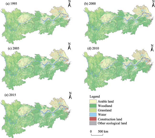
Fig. 4 Spatial pattern of ecological lands in the YREB from 1995 to 2015

4.2 The extent of ecological land change

Table 5 shows the areas of the five types of ecological land change in the YREB from 1995 to 2015. In the past 20 years, the total damaged area was larger than the total recovered area; while the area of unchanged ecological land was the largest, accounting for 84.16%; and the areas of slight damage and slight recovery accounted for 7.93% and 7.29%, respectively. Especially from 2010 to 2015, the area of the severe damage type was larger than the slight recovery type. The area of ecological land damage during this period was clearly much larger than the restored area, and the ecological land was seriously damaged.
Table 5 Areas of ecological land changes in the YREB (km2)
Stages Severe damage Slight damage Unchanged Slight recovery Obvious recovery
1995‒2015 9053 161490 1713018 148307 3513
1995‒2000 3805 149134 1731878 146935 3511
2000‒2005 881 6525 2138318 3400 65
2005‒2010 677 4119 2043259 1289 26
2010‒2015 3433 8474 2035341 2006 220
Table 6 shows the areas of ecological land changes in different regions in the YREB from 1995 to 2015. Similar to the overall trend, the upstream, midstream, and downstream regions were dominated by unchanged types. The upstream area is the largest, but its area of obvious recovery is the smallest. On the contrary, the downstream area is the smallest, but its area of obvious recovery is the largest. To a certain extent, this reflects the differences in the importance and policies of ecological land protection in different regions.
Table 6 Areas of ecological land changes in different regions in the YREB from 1995 to 2015 (km2)
Regions Severe damage Slight damage Unchanged Slight recovery Obvious recovery
Upstream 2477 87028 942775 84836 943
Midstream 3303 35974 480717 33635 1142
Downstream 3253 38475 259397 29839 1428
Figure 5 shows the spatial distribution of the five levels of ecological land change in the YREB from 1995 to 2015. The spatial pattern of ecological lands in the YREB has undergone great changes in the past 20 years. The ecological land changes were mainly in the categories of slight damage and slight recovery, followed by severe damage, and the area of obvious recovery was the smallest. In the upstream region, the ecological land showing slight damage and slight recovery had a similar pattern in spatial distribution, mainly in the southern regions of the Yangtze River, such as Yunnan, Guizhou, etc. In the midstream region, the ecological land showing slight damage and slight recovery was mainly distributed in Hunan Province. While in the downstream area, the ecological land showing slight damage and slight recovery are distributed in north and south, mainly including Anhui, Zhejiang and other regions. There were fewer areas with severe damage or obvious recovery, and their distributions were relatively scattered, showing no obvious spatial distribution pattern. In addition, the conversion of non- ecological land to complete ecological land was very rare. The areas of ecological land change in Sichuan in the north of the upstream of the Yangtze River, Jiangxi and Hubei in the midstream, and Jiangsu in the downstream were generally less than in other places, indicating that the protection of ecological land in these areas was relatively stable.
Figure 5 shows characteristic areas with the four types of ecological land change at a scale of 1:125000. In Fig. 5(a) and Fig. 5(d), the most obvious types are severe damage and obvious recovery, respectively. These types have the smaller areas and more scattered distributions, and they are basically mixed with the other types spatially. In Fig. 5(b) and Fig. 5(c), the types are mainly slight damage and slight recovery, respectively.
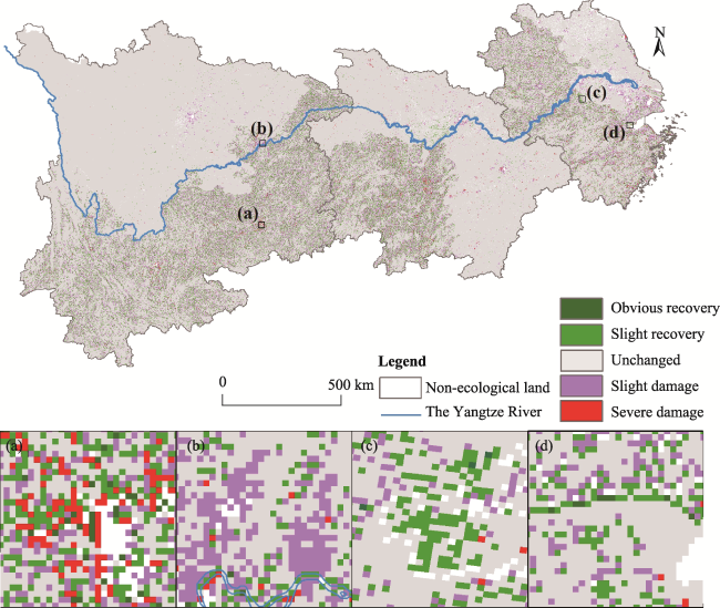
Fig. 5 Spatial distribution of types of ecological land damage in the YREB from 1995 to 2015 Note: (a), (b), (c) and (d) mainly show severe damage, slight damage, slight recovery and obvious recovery, respectively.
Table 7 shows the areas of conversion between the six land types in the YREB from 1995 to 2015. Slight damage mainly includes conversion of complete ecological land to semi-ecological land and semi-ecological land to non-ecological land; while slight recovery mainly includes conversion of non-ecological land to semi-ecological land and semi-ecological land to complete ecological land. In the past 20 years, the main land use changes characterized as slight damage were the conversions of woodland to arable land and arable land to construction land, which accounted for 59.43 % and 18.07 %, respectively. The main changes in land use types for slight recovery of ecological land were the conversion of arable land to woodland, as well as grassland and construction land to arable land. The proportions of these three are 66.67 %, 18.53 % and 8.08 %, respectively.
Table 7 The area transition matrix of ecological land in the YREB from 1995 to 2015 (km2)
Land types Semi-ecological land Complete ecological land Non-ecological land
2015
1995
Arable land Woodland Grassland Water Other ecological land Construction land
Arable land - 98872 27475 9664 312 29177
Woodland 95973 - 57989 3973 780 5790
Grassland 28806 55389 - 1587 671 1507
Water 7308 3242 1032 - 414 1737
Other ecological land 226 565 707 672 - 19
Construction land 11984 2103 532 853 25 -
Figure 6 shows the spatial characteristics of ecological land changes at the municipal level in the YREB from 1995 to 2015. In terms of the damage aspect, the greatest damage was in arable land, followed by woodland and grassland. From Fig. 6, only a few areas of arable land area have increased in the past 20 years, mainly in the southern part of the Yangtze River. In most areas, arable land has been reduced, and the closer to the downstream of the Yangtze River, the greater the area of arable land damage. Grassland in the upstream of the Yangtze River was more severely damaged, while woodland shows the opposite condition. The upstream of the Yangtze River had more recovered areas. Water in most regions has increased, and it only decreased in a few cities. The decrease in water area is much smaller than the increase. For other ecological land types, the areas of most regions did not change much, and the areas with changes mainly showed increases.
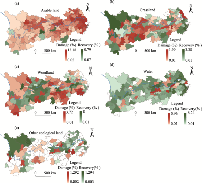
Fig. 6 Spatial characteristics of ecological land change for 130 cities from 1995 to 2015 Note: Red, green, and white indicate the percentages of the damaged area, the recovered area, and the unchanged area of a land type in the total administrative area, respectively.

4.3 Analysis of driving factors

4.3.1 Global effects—Geographic detector
(1) Factor detector
The factor detector mainly measures the explanatory power (q-statistic) of each driving factor for the ecological land change. The larger the q value, the stronger the explanatory power of the driving factor of the ecological land change. The results of the factor detector are shown in Table 8. The average q value is 0.1608, which means that the 14 driving factors explain about 16.08 % of the ecological land change. According to the average q value, the order of the driving factors by explanatory power is: year-end balance of savings of urban and rural residents (B5) > total investment in fixed asset (C2) > proportion of the tertiary industry in the regional GDP (C5) > proportion of the secondary industry in the regional GDP (C4) > urbanization level (B1) > development scale (B3) > annual average temperature (A4) > annual average precipitation (A3) > total retail sales of social consumer goods (C3) > urban road density (B4) > slope (A2) > GDP (C1) > population density (B2) > elevation (A1).
Table 9 further shows the relationships between the driving factors and five types of land, and the effects of most driving factors on a single land type are not significant. The factor detector is better for exploring the global effects. Therefore, in this study, a geographically weighted regression model is used to assess the local effects of the driving factors in Section 4.3.2.
Table 8 Results of the factor detector
Classes First-level indicators Basic-level indicators Rank q value P value
Natural factors (A) Topography A1 Elevation 14 0.0568 0.2379
A2 Slope 11 0.1338 0.0176*
Climate A3 Annual average precipitation 8 0.1598 0.0031**
A4 Annual average temperature 7 0.1599 0.0046**
Social factors (B) Urbanization level B1 Proportion of non-agricultural population to total
population
5 0.1650 0.0024**
Population B2 Population density 13 0.1302 0.0109*
Development scale B3 Proportion of construction land to the total area of the city 6 0.1635 0.0110*
Infrastructure B4 Urban road density 10 0.1572 0.0057**
Savings level (Social Stability Index) B5 Year-end balance of savings of urban and rural residents 1 0.2700 0.0470*
Economic factors (C) The level of economic development C1 GDP 12 0.1316 0.0550
C2 Total investment in fixed assets 2 0.2078 0.1998
Consumption level C3 Total retail sales of social consumer goods 9 0.1582 0.0594
Industrial structure C4 Proportion of the secondary industry in the regional GDP 4 0.1754 0.0025**
C5 Proportion of the tertiary industry in the regional GDP 3 0.1826 0.0021**

Note: * P<0.05, indicates statistical significance at the 5% level; **P<0.01, indicates statistical significance at the 1% level.

Table 9 Factor detector results of the five land type
Basic-level indicators Arable land Woodland Grassland Water Other ecological land
Elevation (A1) 0.0675 0.0088 0.0243 0.0754 0.0176
Slope (A2) 0.1326 0.0611 0.0383 0.0436 0.0229
Annual average precipitation (A3) 0.2396*** 0.0213 0.0068 0.0128 0.0189
Annual average temperature (A4) 0.1696* 0.0089 0.0259 0.0085 0.0099
Proportion of non-agricultural population to total population (B1) 0.2700*** 0.0132 0.0092 0.0537 0.01095
Population density (B2) 0.2838* 0.0007 0.0140 0.0408 0.0072
Proportion of construction land to the total area of the city (B3) 0.1116* 0.0377 0.0307 0.0414 0.0176
Urban road density (B4) 0.1821** 0.0268 0.0011 0.0152 0.0236
Year-end balance of savings of urban and rural residents (B5) 0.0597 0.0518 0.0712 0.0924 0.0074
GDP (C1) 0.0667 0.0640 0.0876 0.0661 0.0071
Total investment in fixed assets (C2) 0.0719 0.0070 0.0318 0.0299 0.0196
Total retail sales of social consumer goods (C3) 0.0569 0.0687 0.0517 0.0646 0.0107
Proportion of the secondary industry in the regional GDP (C4) 0.2355*** 0.0499 0.0032 0.0660 0.0424
Proportion of the tertiary industry in the regional GDP (C5) 0.2106*** 0.0232 0.0113 0.0508 0.0221

Note: *P<0.05, indicates statistical significance at the 5 % level; ** P<0.01, indicates statistical significance at the 1 % level; ***P<0.001, the independent variable is significantly related to the dependent variable.

(2) Risk detector
The risk detector in the geographic detector is used to judge whether the influences of each driving factor on ecological land change are different. Fig. 7 shows that there are two types of relationships between the driving factors and ecological land, i.e., linear effects and nonlinear effects. The results show that the influence of socio-economic factors on the ecological land change is more complicated than that of natural factors, when comparing the differences of driving factors between the subregions.
Fig. 7 The risk detector of the driving factors for the ecological land change Note: The X-axis is the subregion of driving factors; the Y-axis is the area of ecological land change (km2). A1-Elevation, A2-Slope, A3-Annual average precipitation, A4-Annual average temperature, B1-Proportion of non-agricultural population to total population, B2-Population density, B3-Proportion of construction land to the total area of the city, B4-Urban road density, B5-Year-end balance of savings of urban and rural residents, C1-GDP, C2-Total investment in fixed assets, C3-Total retail sales of social consumer goods, C4-Proportion of the secondary industry in the regional GDP, C5-Proportion of the tertiary industry in the regional GDP.
First, the natural factors such as elevation (A2) have apparently nonlinear effects on the ecological land change at the subregion level; whereas the effects of the slope (A2), annual average precipitation (A3), and annual average temperature (A4) on the ecological land change are monotonically increasing (linear) at the subregion level. Second, in terms of the socio-economic factors, the relationships between most driving factors and the ecological land change are close to monotonically increasing, except for year-end balance of savings of urban and rural residents (B5) and GDP (C1).
(3) Interaction detector
Table 10 shows the q-values of the interaction detector. These values show that the explanatory power (interactive effect) between any two driving factors (i.e., the q values in the off-diagonal cells) is always greater than that of a single individual driving factor to the ecological land change (i.e., the q value in the diagonal cells). Furthermore, the interaction relationship is mainly expressed as nonlinear enhance (13 pairs, accounting for 14.29%) and bi-enhance (78 pairs, accounting for 85.71%). First, in terms of nonlinear enhance, the explanatory power has a maximum value of 0.4821 (A1∩B3) and a minimum value of 0.2630 (A1∩B2). Second, in terms of bi-enhance, the maximum value of the explanatory power is 0.3264 (B4∩B5), whereas the minimum value is 0.1494 (A2∩B2). These results show that, to some extent, the interactions between the natural factors and the socio-economic factors can enhance the explanatory ability of the driving factors for the ecological land change.
Table 10 The explanatory power between any two driving factors
Indicators A1 A2 A3 A4 B1 B2 B3 B4 B5 C1 C2 C3 C4 C5
A1 0.057
A2 0.368 0.134
A3 0.424 0.178 0.160
A4 0.413 0.186 0.179 0.160
B1 0.408 0.180 0.176 0.179 0.165
B2 0.263 0.149 0.173 0.173 0.175 0.130
B3 0.482 0.189 0.176 0.178 0.176 0.175 0.163
B4 0.392 0.169 0.196 0.204 0.191 0.169 0.214 0.157
B5 0.441 0.302 0.291 0.300 0.293 0.286 0.301 0.326 0.270
C1 0.384 0.160 0.174 0.185 0.178 0.152 0.195 0.185 0.295 0.132
C2 0.377 0.232 0.239 0.258 0.251 0.224 0.247 0.241 0.286 0.249 0.208
C3 0.477 0.196 0.174 0.179 0.178 0.173 0.176 0.204 0.290 0.229 0.266 0.158
C4 0.464 0.215 0.192 0.186 0.188 0.185 0.188 0.242 0.308 0.220 0.282 0.194 0.175
C5 0.477 0.239 0.197 0.193 0.194 0.192 0.201 0.273 0.311 0.229 0.289 0.201 0.194 0.183

Note: The diagonal q values represent the explanatory power of the individual driving factors, whereas the off-diagonal q values represent the interactions between pairs of the driving factors.

4.3.2 Local effects—Geographically weighted regression
Since the q statistic of the geographical detector can only assess the explanatory power of the driving factors on the ecological land change, we further used the geographically weighted regression tool to quantify the local positive and negative effects of the driving factors, which are represented by the sign and magnitude of the estimated regression coefficients of the geographically weighted regression. As shown in Table 11, all driving factors have both positive and negative effects on the ecological land change at the local scale. While the four largest average local effects are: slope (A2), annual average temperature (A4), proportion of non-agricultural population to total population (B1), and total retail sales of social consumer goods (C3); the four negative driving factors are: proportion of construction land to the total area of the city (B3), year-end balance of savings of urban and rural residents (B5), GDP (C1), and total investment in fixed assets (C2).
Table 11 Descriptive statistics for the regression coefficients of the geographically weighted regression model
Indicators Min Max Mean Q1 Median Q3 STD
Elevation (A1) ‒0.07 ‒0.04 ‒0.05 ‒0.06 ‒0.06 ‒0.05 0.01
Slope (A2) 0.04 0.07 0.05 0.05 0.05 0.06 0.01
Annual average precipitation (A3) ‒0.05 0.04 ‒0.01 ‒0.04 ‒0.02 0.01 0.02
Annual average temperature (A4) 0.01 0.09 0.05 0.03 0.05 0.07 0.02
Proportion of non-agricultural population to total population (B1) 0.01 0.07 0.04 0.02 0.04 0.05 0.01
Population density (B2) ‒0.10 ‒0.05 ‒0.07 ‒0.09 ‒0.08 ‒0.06 0.01
Proportion of construction land to the total area of the city (B3) ‒0.33 ‒0.14 ‒0.21 ‒0.25 ‒0.20 ‒0.17 0.05
Urban road density (B4) ‒0.06 ‒0.05 ‒0.05 ‒0.05 ‒0.05 ‒0.05 0
Year-end balance of savings of urban and rural residents (B5) ‒0.53 ‒0.13 ‒0.30 ‒0.41 ‒0.28 ‒0.20 0.11
GDP (C1) ‒0.65 0.04 ‒0.39 ‒0.55 ‒0.43 ‒0.22 0.18
Total investment in fixed assets (C2) ‒0.59 ‒0.51 ‒0.54 ‒0.56 ‒0.54 ‒0.52 0.02
Total retail sales of social consumer goods (C3) 0.31 0.48 0.43 0.40 0.45 0.47 0.04
Proportion of the secondary industry in the regional GDP (C4) ‒0.04 0.00 ‒0.02 ‒0.03 ‒0.02 ‒0.01 0.01
Proportion of the tertiary industry in the regional GDP (C5) ‒0.01 0.01 0 0 0 0 0

Note: Q1 represents the Lower Quartile; Q3 represents the Upper Quartile; STD represents the Standard Deviation.

In order to further explore the spatial variation characteristics of the driving factors for ecological land changes, our study uses ArcMap 10.5 software to visualize the estimation results and significance of the regression coefficients of the GWR model (Fig. 8). The influences of the driving factors for ecological land change are different in different regions. For example, among the natural factors, elevation has a negative effect on ecological land change, and it gradually increases from northwest to southeast in the YREB. Terrain is high in the west and low in the east. The negative impact of higher elevation on ecological land change is relatively weak, whereas the slope has a positive effect on the ecological land change, and that effect gradually increases from the upstream and downstream of the Yangtze River to the midstream. For the socio-economic factors, urbanization level has a positive effect on the ecological land change, and that effect gradually increases from the northwest to the southeast. The effects of population density and urbanization level have opposite trends, with population density having a negative effect on the ecological land change.
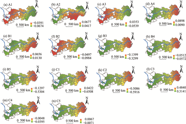
Fig. 8 Spatial distribution of regression coefficients of driving factors Note: A1-Elevation, A2-Slope, A3-Annual average precipitation, A4-Annual average temperature, B1-Proportion of non-agricultural population to total population, B2-Population density, B3-Proportion of construction land to the total area of the city, B4-Urban road density, B5-Year-end balance of savings of urban and rural residents, C1-GDP, C2-Total investment in fixed assets, C3-Total retail sales of social consumer goods, C4-Proportion of the secondary industry in the regional GDP, C5-Proportion of the tertiary industry in the regional GDP.

5 Discussion

Our study analyzed the spatial pattern and driving factors of ecological land change, and obtained results similar to those of both Yuan et al. (2019) and Ran and Li (2020), in that the area of ecological land showed a downward trend from 1995 to 2015. Hu and Zou (2020) discussed the driving factors for ecological land use changes in the YREB, and also believed that government policies, industrial structure and human activities have an impact on changes in ecological land use.

5.1 Path to reducing the ecological land damage in China

Based on the above analysis of the temporal and spatial characteristics of ecological land change and its driving factors, we propose some specific ways to try to reduce the ecological land damage in the study area. The proposed path includes the following three aspects.
The first aspect is the coordinated development of land use and ecological land protection. The spatial pattern and change analysis in this study show that the area of ecological land was generally decreasing. Human activities are the main factor affecting land use, and the rapid urbanization and expansion of construction land crowd out ecological land. In addition, the driving factor analysis of our study shows that interactions between the natural factors and the socio-economic factors can enhance the explanatory ability of the driving factors for the ecological land change. Therefore, local governments need to coordinate the relationships between land use development and ecological land protection (Yu, 2016). We should insist on giving priority to ecology, protect ecological land (Lin, 2016), and further achieve the coordinated development of production, life, and ecology.
The second aspect is the implementation of zoning control for ecological land protection. Our study shows that ecological land change, and the influence of the factors driving it, are different in different regions, and it varies considerably from region to region. Currently, China is working to establish a regional ecological environment management and control system, and 11 provinces (cities) in the YREB are important pilot areas. Chongqing, Zhejiang, Shanghai, Jiangsu, Sichuan, Anhui and Hunan have successively issued the “san xian yi dan (三线一单)”( “san xian yi dan” refers to the ecological protection red line, the environmental quality baseline, the resource utilization baseline, and the ecological environment access list.) ecological environment zoning management and control plan. Each region should consider its own characteristics and establish a regional management and control system for ecological land protection in accordance with the characteristics of the regional social and economic development. Ecological land protection is an important task for promoting the high-quality development.
The third aspect is that the government should not only strengthen the planning of the YREB, but also improve the legislation related to the regulation and protection of ecological land (Wang, 2012). In 2016, the Political Bureau of the CPC Central Committee proposed “Outline of Yangtze River Economic Belt Development”. This outline proposed to vigorously protect the ecological environment of the Yangtze River, and to drive industrial transformation and upgrading through innovation. The analysis of driving factors in our study shows that the proportion of the secondary and tertiary industries has a great impact on the ecological land change, underscoring the importance of transforming the industrial structure. As for legal considerations, although China has issued a series of laws on ecological land protection, such as “Soil and Water Conservation Law”, “Environmental Protection Law”, “Forestry Law”, “Water Resources Law”, and “Grassland Law”, the legal system for ecological land protection is still not sound enough. The existing laws and regulations are especially inadequate in the process of implementation, while the supporting mechanisms are not perfect, which affects the ultimate effectiveness of the protection of ecological land (Wang, 2018). In addition, the government should also pay attention to improving the relevant laws and regulations related to ecological compensation, so that ecological compensation, especially regional ecological compensation, will be legalized and standardized (Wang, 2012).

5.2 Limitations

Our research still has many shortcomings. On the one hand, due to the limitations of remote sensing data availability, only the data from 1995 to 2015 could be used in this study, and the assessment over longer periods of time should be strengthened. On the other hand, our study only assessed the spatial and temporal evolution of the quantitative structure and spatial pattern of ecological land change, and discussed the effects of 14 driving factors on ecological land change. In the future, the dynamic simulation and prediction of ecological land change should be further strengthened based on scenario analysis in the study area.

6 Conclusions

Based on five periods of land use data from 1995 to 2015, our study assessed the extent of ecological land change and its spatial pattern in the YREB, and further explored the global effects and the local effects of 14 driving factors on ecological land change by using the geographical detector and GWR model, respectively.
From 1995 to 2015, the area of ecological land in study area initially increased and then decreased, with an overall decreasing trend. Arable land and woodland were the main types of land area showing decline, in particular, the area of arable land had decreased significantly. In contrast, the areas of grassland, water and other ecological land had increased slightly. In terms of the ecological land damage over the past 20 years, the type of unchanged was dominant, followed by the slight damage and slight recovery types. The total damaged area of ecological land was greater than the area of recovery.
The geographical detector was used to explore the explanatory power of driving factors for ecological land change on the global level, and the GWR model was used to detect the positive/negative local effects of driving factors on ecological land change. Ecological land change is the net result of the interaction of many driving factors, and the explanatory power between any two factors is greater than each single factor. In addition, for different geographical locations, driving factors have different impacts on ecological land change.
1
Bajzak D, Roberts B A . 1996. Development of ecological land classification and mapping in support of forest management in northern Newfoundland, Canada. Environmental Monitoring and Assessment, 39: 199‒213.

2
Belmeziti A, Cherqui F, Kaufmann B . 2018. Improving the multi- functionality of urban green spaces: Relations between components of green spaces and urban services. Sustainable Cities and Society, 43: 1‒10.

3
Bruce E M, Randal G P . 1996. Developing an ecological land classification for the Fundy model forest, southeastern New Brunswick, Canada. Environmental Monitoring and Assessment, 39: 149‒172.

4
Chen L . 2015. Study on provincial tourism competitiveness based on niche theory: A case study on Yangtze River Economic Belt. Diss., Wuhan, China: Central China Normal University. (in Chinese)

5
Chen L, Zhou S L, Zhou B B , et al. 2015. Characteristics and driving forces of regional land use transition based on the leading function classification: A case study of Jiangsu Province. Economic Geography, 35(2): 155‒162. (in Chinese)

6
Costanza R, Daly H E . 1992. Natural capital and sustainable development. Conservation Biology, 6(1): 37‒46.

7
Costanza R, d’Arge R, de Groot R , et al. 1997. The value of the world’s ecosystem services and natural capital. Nature, 387: 253‒260.

8
Cui D . 2015. Research in driving factors of land urbanization in Yangtze River DeIta Area. Diss., Wuhan, China: Huazhong University of Science & Technology. (in Chinese)

9
Dang L J, Xu Y, Gao Y . 2014. Assessment method of functional land use classification and spatial system—A case study of Yangou Watershed. Research of Soil and Water Conservation, 21(5): 193‒197, 203. (in Chinese)

10
Deng H B, Chen C D, Liu X , et al. 2009. Conception and function classification of regional ecological land. Acta Ecologica Sinica, 29(3): 1519‒1524. (in Chinese)

11
Ding L, Xia H H, Shi Y , et al. 2020. Evolution of industrial structure and its environmental effect in the Yangtze River Economic Belt from 2000 to 2015. Safety and Environmental Engineering, 27(2): 8‒1. (in Chinese)

12
Dong Y W, Zhou W, Zhou L , et al. 1999. Research on ecological protection in urban areas. Urban Research,(2): 6‒8,10. (in Chinese)

13
Fang C L, Zhou C H, Wang Z B . 2015. Sustainable development strategy and priorities of spatially differentiated development of urban agglomerations along the Yangtze River Economic Belt. Progress in Geography, 34(11): 1398‒1408. (in Chinese)

DOI

14
Fei J B, Xia J G, Hu J , et al. 2019. Research progress of ecological space and ecological land in China. Chinese Journal of Eco-Agriculture, 27(11): 1626‒1636. (in Chinese)

15
Grondin P, Gauthier S, Borcard D , et al. 2014. A new approach to ecological land classification for the Canadian boreal forest that integrates disturbances. Landscape Ecology, 29(1): 1‒16.

DOI

16
Hu J T. 2012. Report of the 18th Party Congress. Beijing, China: People’s Publishing House.

17
Hu X D, Zou L L . 2020. Landscape pattern evolution of land use and its driving mechanism in Yangtze River Economic Belt under the guidance of ecological priority: Case study of Wuhan City. Areal Research and Development, 39(3): 138‒149. (in Chinese)

18
Hu X J, Gao L, Ma C M , et al. 2020. Land use zoning of Weifang North Plain based on ecological function and geo-environmental suitability. Bulletin of Engineering Geology and the Environment, 79(5): 2697‒2719.

19
Huang J C, Lin H X, Qi X X . 2017. A literature review on optimization of spatial development pattern based on ecological-production-living space. Progress in Geography, 36(3): 378‒3.1. (in Chinese)

20
Jiang W Y, Cai Y L, Tian J J . 2019. The application of minimum cumulative resistance model in the evaluation of urban ecological land use efficiency. Arabian Journal of Geosciences, 12(23): 1‒7.

21
Jozi S A, Majd N M . 2015. Ecological land capability evaluation of Dehloran County in order to ecotourism development. Journal of the Indian Society of Remote Sensing, 43(3): 571‒581.

22
Klijn F, Haes H A U D. 1994. A hierarchical approach to ecosystems and its implications for ecological land classification. Landscape Ecology, 9(2): 89‒104.

23
Li D J, Xu E Q, Zhang H Q . 2020. Influence of ecological land change on wind erosion prevention service in arid area of northwest China from 1990 to 2015. Ecological Indicators, 117. DOI: 10.1016/j.ecolind.2020.106686.

24
Li G D, Fang C L, Wang S J , et al. 2016. Progress in remote sensing recognition and spatio-temporal changes study of urban and rural land use. Journal of Natural Resources, 31(4): 703‒718. (in Chinese)

25
Li Y, Feng Y, Peng F , et al. 2017. Pattern evolvement of ecological land in Tianjin based on geographic detector. Economic Geography, 37(12): 180‒189.

26
Lin H R, Feng Y F . 2018. Identification and analysis of “production-living-ecological space” of Xiajie Village, Zhanjiang City, Guangdong Province. Journal of Guangzhou University (Natural Science Edition), 17(1): 82‒87, 94. (in Chinese)

27
Lin X L . 2016. Analysis on time space process and driving factors for ecological land loss in the urban circle of Wuhan. Diss., Wuhan, China: South-Central University for Nationalities. (in Chinese)

28
Liu D Q, Ma X C, Gong J , et al. 2018. Functional identification and spatiotemporal pattern analysis of production-living-ecological space in watershed scale: A case study of Bailongjiang Watershed in Gansu. Chinese Journal of Ecology, 37(5): 1490‒1497. (in Chinese)

29
Liu F, Zhang H Q . 2016. Ecological land use mapping and spatio-temporal dynamics in the Tarim Basin. Resources Science, 38(5): 825‒836. (in Chinese)

30
Liu J L, Liu Y S, Li Y R . 2017a. Classification evaluation and spatial-temporal analysis of “production-living-ecological” spaces in China. Acta Geographica Sinica, 72(7): 1290‒1304. (in Chinese)

31
Liu S H, Wang D Y, Li H , et al. 2017b. Ecological land fragmentation evaluation and dynamic change of a typical black soil farming area in Northeast China. Sustainability, 9(2):300. DOI: 10.3390/su9020300.

32
Liu Y W, Liu C W, He Z Y , et al. 2020. Spatial-temporal evolution of ecological land and influence factors in Wuhan urban agglomeration based on geographically weighted regression model. Chinese Journal of Applied Ecology, 31(3): 987‒998. (in Chinese)

PMID

33
Long H R . 2015. The changes of ecological land in Chang-Zhu-Tan region and its effect mechanism. Diss., Changsha, China: Central South University of Forestry and Technology. (in Chinese)

34
Naser A S, Sasan B K, Timo P , et al. 2016. Integrated use of GIS, remote sensing and multi-criteria decision analysis to assess ecological land suitability in multi-functional forestry. Journal of Forestry Research, 27(5): 1127‒1135.

35
Peng J, Wang A, Liu Y X , et al. 2015. Research progress and prospect on measuring urban ecological land demand. Acta Geographica Sinica, 70(2): 333‒346. (in Chinese)

36
Peng J, Zhao M Y, Guo X N , et al. 2017. Spatial-temporal dynamics and associated driving forces of urban ecological land: A case study in Shenzhen City, China. Habitat International, 60: 81‒90.

37
Peng K F, Jiang W G, Deng Y . 2019. Identification of wetland damage degree and analysis of its driving forces in Wuhan Urban Agglomeration. Journal of Natural Resources, 34(8): 1694‒1707. (in Chinese)

38
Ran R, Li J F . 2020. Transformation of land use and ecological environment effect in the Yangtze River Economic Belt. Jiangsu Agricultural Sciences, 48(2): 256‒263. (in Chinese)

39
Rowe J S, Sheard J W . 1981. Ecological land classification: A survey approach. Environmental Management, 5(5): 451‒464.

40
Sun D F . 2005. Analysis of socio-economic driving forces on land desertification at Minqin County in Gansu Province in 1988‒1997. Transactions of the Chinese Society of Agricultural Engineering, 21(S1): 131‒135. (in Chinese)

41
Tan Y Z, Zhao Y, Cao Y , et al. 2016. Research progress on regional ecological land classification in China. China Land Sciences, 30(9): 28‒36. (in Chinese)

42
Tang A, Li X S, Bian Z F , et al. 2016. Research on the driving factors of the ecological land evolution based on data reconstruction: A case study of the southwest coal cities. Ecological Economy, 32(5): 136‒142. (in Chinese)

43
Tu J, Xia Z G . 2008. Examining spatially varying relationships between land use and water quality using geographically weighted regression I: Model design and evaluation. Science of the Total Environment, 407(1): 358‒378.

44
Wang H . 2018. Study on the ecological land change and management strategy of Zhejiang Province. Diss., Hangzhou, China: Zhejiang Gongshang University. (in Chinese)

45
Wang J F, Xu C D . 2017. Geodetector: Principle and prospective. Acta Geographica Sinica, 72(1): 116‒134. (in Chinese)

46
Wang J Z . 2012. Study on ecological land change and the driving force in Poyang Lake ecological economic region. Diss., Nanchang, China: Jiangxi University of Finance & Economics. (in Chinese)

47
Wang L P, Chen J . 2016. Socio-economic influential factors of haze pollution in China: Empirical study by EBA model using spatial panel data. Acta Scientiae Circumstantiae, 36(10): 3833‒3839. (in Chinese)

48
Wang Z B, Luo K, Song J , et al. 2015. Characteristics of change and strategic considerations of the structure of urban functional divisions in the Yangtze River Economic Belt since 2000. Progress in Geography, 34(11): 1409‒1418. (in Chinese)

49
Xiao B Y, Dai L M, Chen G , et al. 2002. Application of GIS in ecological land type (ELT) mapping—A case in Changbai Mountain area. Journal of Forestry Research, 13(1): 56‒60.

50
Xiao D N, Li X Z . 1997. Development and prospect of contemporary landscape ecology. Scientia Geographica Sinica, 17(4): 356‒364. (in Chinese)

51
Xie G D, Lu C X, Cheng S K , et al. 2001. Evaluation of natural capital utilization with ecological footprint in China. Resources Science, 23(6): 20‒23. (in Chinese)

52
Xie H L, Li X B . 2011. Analysis of regionally ecological land use and its influencing factors based on a logistic regression model in the Beijing-Tianjin-Hebei Region, China. Resources Science, 33(11): 2063‒ 2070. (in Chinese)

53
Xie H L, Liu Z F, Wang P , et al. 2013. Exploring the mechanisms of ecological land change based on the spatial autoregressive model: A case study of the Poyang Lake Eco-Economic Zone, China. International Journal of Environmental Research and Public Health, 11(1): 583‒599.

DOI PMID

54
Yu F, Li X B, Zhang L J , et al. 2015. Study of ecological land in China: Conception, classification, and spatial-temporal pattern. Acta Ecologica Sinica, 35(14): 4931‒4943. (in Chinese)

55
Yu L, Song A A, Zheng Y , et al. 2017. The ecological-living-industrial land classification system and the analysis of its spatial distribution—Case of Changli County. Chinese Journal of Agricultural Resources and Regional Planning, 38(2): 89‒96. (in Chinese)

56
Yu X F . 2016. Study on the land use and land cover change and its driving forces based on RS and GIS—Setting Jiangbei District of Chongqing as the example. Diss., Chongqing, China: Southwest University. (in Chinese)

57
Yuan S F, Tang Y Y, Shentu C N . 2019. Spatiotemporal change of land-use transformation and its eco-environmental response:A case of 127 counties in Yangtze River Economic Belt. Economic Geography, 39(9): 174‒181. (in Chinese)

58
Zeng C Y, Yang L, Zhu A X , et al. 2016. Mapping soil organic matter concentration at different scales using a mixed geographically weighted regression method. Geoderma, 281: 69‒82.

59
Zhang H Q, Wang L X, Jia B Q . 2004. A conception of ecological land use and its function classification in arid area in Northwest China. Chinese Journal of Eco-Agriculture, 12(2): 5‒8. (in Chinese)

60
Zhang H Q, Xu E Q, Zhu H Y . 2017a. Ecological-Living-Productive land classification system in China. Journal of Resources and Ecology, 8(2): 121‒128.

61
Zhang H, Wang Y . 2017. Spatial differentiation of cropland pressure and its socio-economic factors in China based on panel data of 342 prefectural-level units. Geographical Research, 36(4): 731‒742. (in Chinese)

62
Zhang Q, Gao M, Yang L , et al. 2017b. Changes in the spatial structure of ecological land and ecosystem service values in nine key districts of Chongqing City over the past 25 years. Acta Ecologica Sinica, 37(2): 566‒575. (in Chinese)

63
Zhang W S, Jiang L, Cui Y Z , et al. 2019. Effects of urbanization on airport CO2 emissions: A geographically weighted approach using nighttime light data in China. Resources, Conservation and Recycling, 150:104454. DOI: 10.1016/j.resconrec.2019.104454.

64
Zhang Y C, Zhang B, Jiang X Y . 2007. Research on social and economic driving mechanism of land use/cover change in oasis region. Journal of Anhui Agricultural Sciences, 35(9): 2683‒2684,2755. (in Chinese)

65
Zhang Y Z, Hu Y F, Zhuang D F . 2020. A highly integrated, expansible, and comprehensive analytical framework for urban ecological land: A case study in Guangzhou, China. Journal of Cleaner Production, 268. DOI: 10.1016/j.jclepro.2020.122360.

66
Zheng T, Chen S, Zhang T . 2019. Changes of ecological land and driving factors in urban riverside area: The case of Nanjing section of the Yangtze River. Resources and Environment in the Yangtze Basin, 28(5): 1049‒1.58. (in Chinese)

67
Zhou D, Lin Z L, Lim S H . 2019. Spatial characteristics and risk factor identification for land use spatial conflicts in a rapid urbanization region in China. Environmental Monitoring and Assessment, 191:677. DOI: 10.1007/s10661-019-7809-1.

DOI PMID

68
Zhou R, Wang X J, Su H L , et al. 2015. Identification and security pattern of ecological land in Pingdingshan newly developed area. Acta Ecologica Sinica, 35(6): 2003‒ 2012. (in Chinese)

69
Zhou Z, Meng J J, Qi Y , et al. 2016. Importance of ecological lands and their pattern optimization in China: A review. Chinese Journal of Ecology, 35(1): 218‒225. (in Chinese)

70
Zhu Z Q, Yang F, Song Z J . 2015. Exploring spatial patterns and complexities of ecological lands in Beijing. Economic Geography, 35(7): 168‒175. (in Chinese)

71
Zou L L, Wang J Y, Hu X D . 2018. A classification systems of production-living-ecological land on the county level: Theory building and empirical research. China Land Science, 32(4): 59‒66. (in Chinese)

Outlines

/