
Journal of Resources and Ecology >
Relationship between Industrialization, Urbanization and Industrial Ecology in Western China: A Panel Vector Auto-Regression Model Analysis
Received date: 2020-06-14
Accepted date: 2020-09-15
Online published: 2021-03-30
Supported by
National Social Science Fundation of China(17XJY020)
National Natural Science Foundation of China(71963028)
Discipline Construction Project for Ningxia Institutions of Higher Education (Discipline of Theoretical Economics)(NXYLXK2017B04)
As the foundation of modern economic development, industry is the engine of industrialized and urbanized development. Industrial ecology is a high-level form of industry that is achieved after it has reached a certain stage, which guides the coordinated industrial development balancing mankind and nature. The implementation of industrial ecology is an important method and effective approach to realize the sustainable development of industrialization and urbanization. In this article, based on the inter-provincial panel data of western China during 2003-2018, the spatial development trends of industrialization, urbanization and industrial ecology are analyzed, and an empirical method is employed to conduct a robustness test based on the Panel Vector Auto-Regression (PVAR) model to determine the long-term interactions among these three aspects. The results show that it is difficult to manifest the short-term causal relationships among industrialization, urbanization and industrial ecology. After lagging for three periods, they present the Granger causality, the industrial ecology and industrialization have promoted urbanization, and the coefficient for the influence of industrial ecology on urbanization is 0.4612. However, industrialization and urbanization have negative impacts on industrial ecology, and with a 1% increase in industrialization or urbanization, the industrial ecology will decline by 0.2261% or 0.2850%, respectively. With the continuation of the lagging period, industrial ecology will have better interpretability than industrialization and urbanization, and industrialization and eco-friendly development have strong self-accumulation development mechanisms, while the self-accumulation mechanism of urbanization is not obvious, and it might even have a decline. By fulfilling the role of the regional leading industry, the state of unbalanced internal development can be improved, so as to realize mutual promotion between industrialization and urbanization. By improving the utilization rates of resources and energy, efforts should be made to implement green production, significantly promote industrial ecology, and boost high-quality development of both the regional economy and society.
Key words: industrialization; urbanization; eco-friendly development; PVAR model
WANG Yajun . Relationship between Industrialization, Urbanization and Industrial Ecology in Western China: A Panel Vector Auto-Regression Model Analysis[J]. Journal of Resources and Ecology, 2021 , 12(1) : 68 -79 . DOI: 10.5814/j.issn.1674-764x.2021.01.007
Table 1 Selection of related industrialization, urbanization and industrial ecology indexes and their weights |
| Destination layer | Criterion layer | Index layer | |||
|---|---|---|---|---|---|
| Economic development level | Per capita GDP (22.9) | ||||
| Industrialization | Economic scale | Proportion of the gross product of tertiary industry in total GDP (18.1) Proportion of labor force population from secondary and tertiary industries in the total labor force population (16.5) | |||
| Government promotion Modernization level of agriculture | Proportion of R&D expenditure in GDP (14.9) Proportions of fiscal revenue and fiscal expenditure (15.4) Total power of agricultural machinery per hectare (12.2) | ||||
| Urbanization | Spatial distribution of population among cities and rural areas | Proportion of urban population in total population (100) | |||
| Industrial development level | Growth speed of industrial added value (21.6) | ||||
| Industrial ecology | Energy and resource utilization | Total energy consumption (17.4) Employment of extractive industry/ Total employment (18.2) | |||
| Environmental pollution degree | Industrial waste water discharge (14.1) Industrial sulfur dioxide emission (14.5) Industrial solid waste utilization rate (14.2) |
Note: For the weights of various indexes within the brackets, the unit is %. |
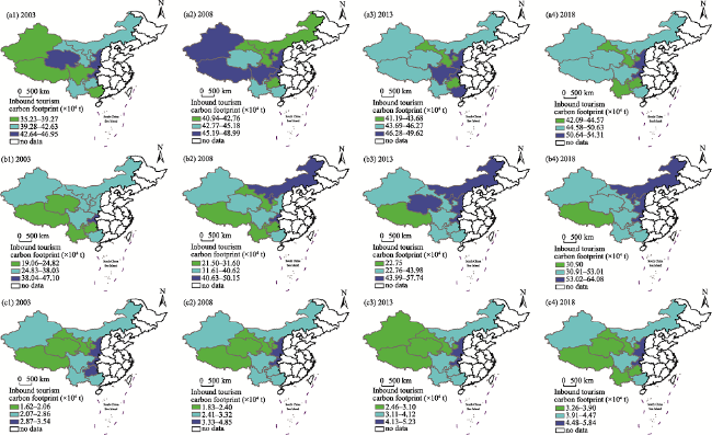
Fig. 1 Spatial distribution of industrialization (a), urbanization (b) and industrial ecology (c) in the western regions |
Table 2 Stationary test of variables |
| Variable | Levin-Lin-Chu (LLC) test statistic value | Augmented Dicey-Fuller (ADF) test statistic value | Result |
|---|---|---|---|
| lnIN | 3.4592 | 8.0304 | Non-stationary |
| lnUR | 2.4235 | 10.0871 | Non-stationary |
| lnEC | 8.7021 | 11.7962 | Non-stationary |
| d_lnIN | -2.9323** | -4.9669** | Stationary |
| d_lnUR | -7.4089** | -10.1276* | Stationary |
| d_lnEC | 0.4426** | -1.2723*** | Stationary |
Note: All the variables in the first three rows of the table are non-stationary. “d_” represents the transformation of variables through first-order difference. *, ** and *** represent the significance levels of statistics at 10%, 5% and 1%, respectively. The LLC test and ADF test of the first-order difference variables were significant, and the non-stationary variables became stationary sequences. |
Table 3 Optimal lagged order test |
| Lag | Bayesian Information Criterion (BIC) | Akaike Information Criterion (AIC) | Hannan Quinn Information Criterion (HQIC) |
|---|---|---|---|
| PVAR(1) | -6.433 | -5.831 | -6.279 |
| PVAR(2) | -7.542 | -3.955 | -4.171 |
| PVAR(3) | -8.496 | -6.548 | -7.098 |
| PVAR(4) | -6.028 | -4.103 | -5.864 |
Note: PVAR(1), PVAR(2), PVAR(3) and PVAR(4) represent the lag orders 1-4 of the PVAR model, respectively. When the lag order is 3, the result shows BIC, AIC and HQIC with the minimum information content, so the lag order should be set as 3. |
Table 4 GMM estimation results of the dynamic panel |
| Variable | h_lnIN | h_lnUR | h_lnEC | |||
|---|---|---|---|---|---|---|
| Coefficient | P value | Coefficient | P value | Coefficient | P value | |
| L1. h_lnIN | 0.7803** | 0.013 | -0.2648 | 0.358 | -0.1818 | 0.582 |
| L1. h_lnUR | 0.6757*** | 0.001 | -0.2436 | 0.226 | 0.3276 | 0.119 |
| L1. h_lnEC | 1.1943*** | 0.000 | -0.2929 | 0.284 | 0.1615 | 0.512 |
| L2. h_lnIN | -0.1011 | 0.541 | -0.0655 | 0.715 | 0.0706 | 0.776 |
| L2. h_lnUR | 0.0173 | 0.917 | 0.1836 | 0.429 | 0.1575* | 0.061 |
| L2. h_lnEC | -0.0161 | 0.920 | -0.0430 | 0.825 | 0.1132 | 0.400 |
| L3. h_lnIN | -0.0916 | 0.346 | 0.0484** | 0.048 | -0.2850* | 0.083 |
| L3. h_lnUR | 0.3333 | 0.114 | 0.1659 | 0.585 | -0.2261*** | 0.004 |
| L3. h_lnEC | -0.0203 | 0.831 | 0.4612*** | 0.009 | -0.0565 | 0.511 |
Note: *, ** and *** represent the significance levels of coefficients at 10%, 5% and 1%, respectively. h_lnIN, h_UR and h_EC are the sequences of lnIN, UR and EC after Helmert conversion to eliminate the individual effects, and L1, L2 and L3 respectively represent the variables of one-period, two-period and three-period lags. Coefficient and P value represent GMM estimated coefficients and estimates, respectively. |
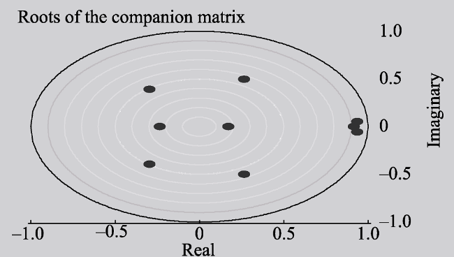
Fig. 2 Stability test |
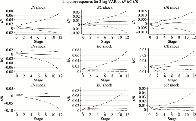
Fig. 3 Impulse response of the impacts of industrialization on urbanization and industrial ecology |
Table 5 Panel Granger Causality Test results |
| Variable | Causality | 2-order lag | 3-order lag | ||||
|---|---|---|---|---|---|---|---|
| Estimated value | Coefficient | Result | Estimated value | Coefficient | Result | ||
| lnIN | lnEC non-Granger cause | 2.698** | 0.041 | Reject | 7.452* | 0.084 | Reject |
| lnUR non-Granger cause | 1.819 | 0.611 | Not reject | 6.308* | 0.092 | Reject | |
| ALL non-Granger cause | 3.952 | 0.683 | Not reject | 9.632* | 0.067 | Reject | |
| lnUR | lnIN non-Granger cause | 2.227 | 0.527 | Not reject | 5.034* | 0.058 | Reject |
| lnEC non-Granger cause | 10.643** | 0.014 | Reject | 3.011*** | 0.000 | Reject | |
| ALL non-Granger cause | 11.723* | 0.068 | Reject | 2.654*** | 0.008 | Reject | |
| lnEC | lnIN non-Granger cause | 5.755 | 0.324 | Not reject | 1.457*** | 0.003 | Reject |
| lnUR non-Granger cause | 2.085 | 0.555 | Not reject | 1.019** | 0.021 | Reject | |
| ALL non-Granger cause | 7.389* | 0.086 | Reject | 5.117** | 0.029 | Reject | |
Note: *, ** and *** represent the significance levels of 10%, 5% and 1%, respectively. |
Table 6 Variance decomposition of the panel error term |
| Variable | Period | lnIN | lnUR | lnEC |
|---|---|---|---|---|
| lnIN | 7 | 0.6231 | 0.0468 | 0.3301 |
| lnUR | 7 | 0.0993 | 0.2554 | 0.6453 |
| lnEC | 7 | 0.1011 | 0.0503 | 0.8486 |
| lnIN | 8 | 0.5549 | 0.0448 | 0.4003 |
| lnUR | 8 | 0.1027 | 0.2431 | 0.6542 |
| lnEC | 8 | 0.0942 | 0.0450 | 0.8608 |
| lnIN | 9 | 0.4987 | 0.0442 | 0.4571 |
| lnUR | 9 | 0.1084 | 0.2335 | 0.6581 |
| lnEC | 9 | 0.0914 | 0.0412 | 0.8673 |
| lnIN | 10 | 0.4544 | 0.0452 | 0.5004 |
| lnUR | 10 | 0.1146 | 0.2270 | 0.6583 |
| lnEC | 10 | 0.0911 | 0.0391 | 0.8698 |
| [1] |
|
| [2] |
|
| [3] |
|
| [4] |
|
| [5] |
|
| [6] |
|
| [7] |
|
| [8] |
|
| [9] |
|
| [10] |
|
| [11] |
|
| [12] |
|
| [13] |
|
| [14] |
|
| [15] |
|
| [16] |
|
| [17] |
|
| [18] |
|
| [19] |
Marx. 1995. Marx and engles anthology (Translated by Compilation and Translation Bureau of the CPC Central Committee). Beijing: People’s Publishing House Press, 217-223. (in Chinese)
|
| [20] |
|
| [21] |
|
| [22] |
|
| [23] |
|
| [24] |
|
| [25] |
|
| [26] |
|
| [27] |
|
| [28] |
|
| [29] |
|
| [30] |
|
/
| 〈 |
|
〉 |